Nuclear physics
🎯What you need to be able to do
- Understand the equivalence between energy and mass, and recall and use \( E = mc^{2} \).
- Represent simple nuclear reactions by nuclear equations, and apply conservation of nucleon number, proton number, mass–energy and momentum.
- Define and use mass defect and binding energy, and binding energy per nucleon.
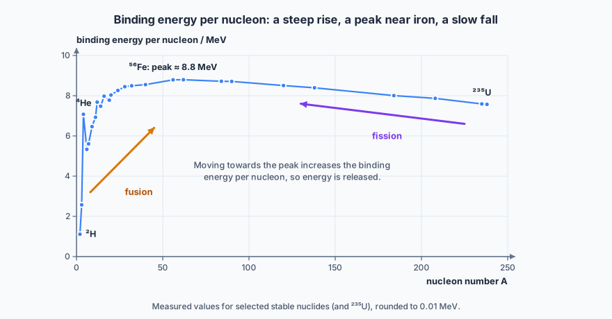
- Sketch the variation of binding energy per nucleon with nucleon number, and explain why energy is released in fission and in fusion.
- Understand that fluctuations in count rate provide evidence for the random nature of radioactive decay.
- Show that the rate of decay is proportional to the number of undecayed nuclei, and define activity and decay constant.
- Use \( A = \lambda N \) and \( x = x_0e^{-\lambda t} \).
- Define half-life and use \( \lambda t_{1/2} = \ln 2 = 0.693 \).
📚The physics
Mass defect. The mass of a nucleus is always less than the sum of the masses of its separate nucleons. The difference, converted by \( E = mc^{2} \), is the binding energy — the energy that would be needed to pull the nucleus apart. It is not stored “in” the nucleus like a spring; the bound system is simply lighter than its parts, which is one of the strangest true statements in the syllabus.
The binding-energy curve rises steeply to a maximum near iron-56, at about 8.8 MeV per nucleon, then falls slowly. Any process that moves nuclei towards the peak releases energy. Light nuclei get there by fusing; heavy ones by splitting. That single curve explains why stars shine and why reactors work, and being able to sketch it — with the peak in the right place and the sharp rise on the left — is directly examinable.
Randomness. No experiment can predict when a particular nucleus will decay, and no external condition — temperature, pressure, chemical state — changes the probability. The evidence is the fluctuation in count rate about a mean, which is why repeat readings of a constant source disagree slightly.
The decay law. Because each nucleus has the same constant probability \(\lambda\) of decaying per unit time, \( \mathrm{d}N/\mathrm{d}t = -\lambda N \), whose solution is \( N = N_0e^{-\lambda t} \). Activity \( A = \lambda N \) follows the same exponential, and so does the count rate. Half-life relates to the decay constant by \( t_{1/2} = \ln 2/\lambda \).
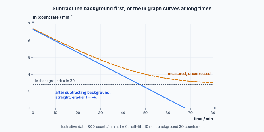
Background must be subtracted from every measured count rate before the decay law is applied. Forgetting it curves an otherwise straight ln-graph at long times, which is a standard Paper 5 discussion point.
✏️Worked example
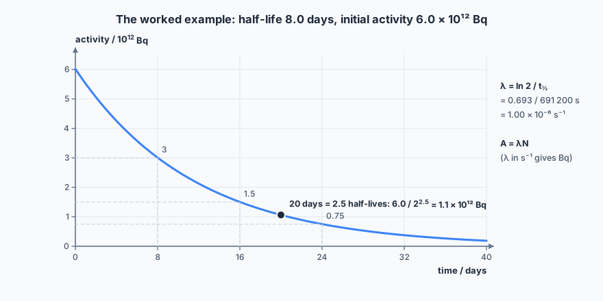
\( \lambda = \ln 2/t_{1/2} = 0.693/(8.0 \times 24 \times 3600) = 1.00 \times 10^{-6} \) s\(^{-1}\).
\( A_0 = \lambda N_0 = 1.00 \times 10^{-6} \times 6.0 \times 10^{18} = 6.0 \times 10^{12} \) Bq.
After 20 days = 2.5 half-lives:
🔭See it happen
Take repeated one-minute counts from a long-lived source and plot the distribution: the spread about the mean is the randomness itself, made quantitative. For half-life, protactinium-234 generators give a measurable decay in about ten minutes, and a dice-shaking simulation with several hundred dice reproduces the exponential convincingly if you have no source at all.
🔗Go deeper — other people’s work
The links below are not mine. They are here because they are good, and they may move or disappear without warning.
- PhET, Alpha Decay and Nuclear Fission.
- IAEA and CERN public pages on binding energy and nuclear structure.
- Isaac Physics, “Nuclear Physics” problem sets.