Graphs of functions and practical graphs
🎯What you need to be able to do
- Use and draw travel and conversion graphs, and interpret the gradient of a straight line as a rate of change.
- Use distance–time and speed–time graphs: acceleration, deceleration, and distance as the area under a speed–time graph EXTENDED.
- Estimate the gradient of a curve by drawing a tangent EXTENDED.
- Complete tables of values and draw graphs of linear, quadratic and reciprocal functions; for Extended also cubics, sums of powers and exponentials \( ab^{x} + c \) EXTENDED.
- Solve equations graphically, including by drawing a straight line.
- Sketch linear and quadratic graphs; for Extended also cubic, reciprocal and exponential graphs with roots, turning points and asymptotes EXTENDED.
📚The mathematics
Practical graphs
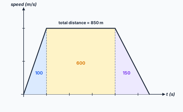
On a distance–time graph the gradient is the speed, and a horizontal section means stopped. On a speed–time graph EXTENDED the gradient is the acceleration (negative gradient: deceleration), and the area under the graph is the distance travelled — split it into triangles, rectangles and trapezia. Watch the units: a graph in minutes and a speed in km/h need converting.
EXTENDED To estimate the gradient of a curve at a point, draw the tangent there with a ruler, pick two points far apart on it, and compute rise over run.
Graphs of functions
Complete the table of values carefully (a calculator helps on Paper 3 and 4 — watch negative \(x\) squared), plot with small crosses, and join with a smooth curve, not straight segments. A quadratic has a rounded bottom (or top), never a point.
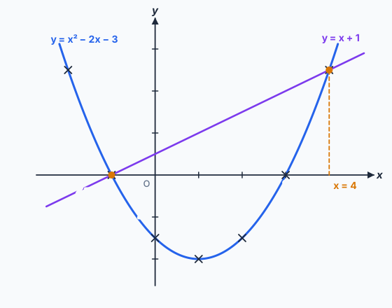
To solve an equation with a graph you already have, rearrange it so one side is the plotted function; the other side is the line to draw. With \( y = x^{2} - 2x - 3 \) drawn, the equation \( x^{2} - 3x - 4 = 0 \) is \( x^{2} - 2x - 3 = x + 1 \): draw \( y = x + 1 \) and read the \(x\)-coordinates of the intersections.
Sketching curves
A sketch shows shape and key features, not plotted points. Label where it crosses the axes, and for a quadratic the turning point (found by completing the square) and line of symmetry.
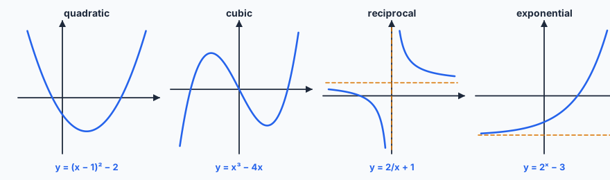
EXTENDED For \( y = \dfrac{a}{x} + b \) the asymptotes are \( x = 0 \) and \( y = b \); for \( y = ar^{x} + b \) the asymptote is \( y = b \) and the \(y\)-intercept is \( a + b \). A cubic \( y = ax^{3} + \ldots \) with \( a > 0 \) goes from bottom left to top right.
✏️Worked example
(a) Acceleration \( = \dfrac{20}{10} = 2 \) m/s². Distance = area \( = \tfrac{1}{2}(10)(20) + 30(20) + \tfrac{1}{2}(15)(20) = 100 + 600 + 150 = 850 \) m.
(b) For \( x = -2, -1, 0, 1, 2, 3, 4 \): \( y = 5, 0, -3, -4, -3, 0, 5 \). Rearranging, \( x^{2} - 3x - 4 = 0 \) is the same as \( x^{2} - 2x - 3 = x + 1 \), so draw \( y = x + 1 \): it meets the curve at \( x = -1 \) and \( x = 4 \).
📝Practise
Questions in the style of the current papers. EXTENDED marks Extended-only content.
1. (Non-calculator.) A conversion graph is a straight line through \( (0, 0) \) and \( (5 \text{ miles}, 8 \text{ km}) \). Convert 45 miles to kilometres. [1]
2. (Non-calculator.) Ana walks 3 km from home in 45 minutes, rests for 15 minutes, then walks home in 30 minutes. Find her speed on the way home, in km/h. [2]
3. (Non-calculator.) EXTENDED A cyclist decelerates uniformly from 24 m/s to rest in 8 s. Find the deceleration and the distance travelled while decelerating. [3]
4. (Calculator.) EXTENDED For \( y = x^{3} - 3x + 1 \), find \(y\) when \( x = -2, 0, 2 \). The graph crosses the \(x\)-axis three times; use it (or trial) to give the roots to 1 decimal place. [4]
5. (Non-calculator.) EXTENDED Write down the equations of the asymptotes of \( y = \dfrac{2}{x} + 1 \), and the asymptote and \(y\)-intercept of \( y = 3 \times 2^{x} - 4 \). [3]
6. (Non-calculator.) EXTENDED By completing the square, sketch \( y = -x^{2} + 4x + 5 \), labelling where it meets the axes and its turning point. [4]
7. (Calculator.) EXTENDED The tangent to \( y = x^{2} \) at \( (3, 9) \) passes through \( (5, 21) \). Find the gradient of the curve at \( x = 3 \). [1]
🔗Go deeper — other people’s work
These are external resources, not mine. If one stops working, tell me and everything above it on this page still stands.
- Desmos — plot a curve and a line together to check graphical solutions
- PhET “The Moving Man” — distance–time and speed–time graphs drawn live