Cumulative frequency and histograms
EXTENDED Everything on this page is Extended content only.
🎯What you need to be able to do
- Complete a cumulative frequency table and draw a cumulative frequency curve.
- Estimate the median, quartiles, interquartile range and percentiles from the curve, and interpret them.
- Calculate frequency density, and draw and interpret histograms with equal or unequal class widths.
📚The mathematics
Cumulative frequency
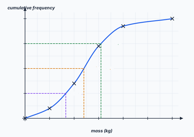
Cumulative frequency is a running total: the number of values up to the end of each class. Plot each running total at the upper boundary of its class (not the midpoint), mark the points with small crosses, start from zero at the lower boundary of the first class, and join them with a smooth curve.
To read the curve with \(n\) values: the median is at \( \tfrac{n}{2} \), the lower quartile at \( \tfrac{n}{4} \), the upper quartile at \( \tfrac{3n}{4} \), and the \(p\)th percentile at \( \tfrac{p}{100} \times n \). Go across from the cumulative frequency axis to the curve, then down. To find how many values are above something, read the curve and subtract from \(n\).
Histograms
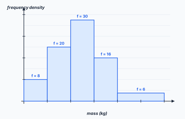
In a histogram the area of each bar, not its height, represents the frequency. The vertical axis is frequency density:
Bars touch (the data are continuous) and their widths match the class widths. When the classes are unequal, a tall bar is not necessarily a large frequency: compare areas.
✏️Worked example
(a) Cumulative frequencies at \( m = 2, 4, 6, 8, 12 \): 8, 28, 58, 74, 80. Plot these (and \( (0, 0) \)) and join with a smooth curve.
(b) Median at \( \tfrac{80}{2} = 40 \): about 4.8 kg. LQ at 20: about 3.3 kg; UQ at 60: about 6.2 kg. IQR \( \approx 6.2 - 3.3 = 2.9 \) kg.
(c) At \( m = 7 \) the curve reads about 68, so about \( 80 - 68 = 12 \) parcels weigh more than 7 kg.
(d) \( 8 \div 2 = 4 \), \( 20 \div 2 = 10 \), \( 30 \div 2 = 15 \), \( 16 \div 2 = 8 \), \( 6 \div 4 = 1.5 \).
📝Practise
All Extended. Questions 3–5 use the parcel data and curve above.
1. (Non-calculator.) A class \( 10 < t \le 25 \) has frequency 45. Find its frequency density. [1]
2. (Non-calculator.) A histogram bar has width 5 and frequency density 2.4. Find the frequency. [1]
3. (Non-calculator.) Use the curve to estimate the 90th percentile of the parcel masses. [2]
4. (Non-calculator.) Estimate how many parcels weigh 3.3 kg or less, and explain the connection with the lower quartile. [2]
5. (Calculator.) Calculate an estimate of the mean mass of the 80 parcels. [3]
6. (Non-calculator.) Two classes sat a test. Class A: median 62, IQR 8. Class B: median 58, IQR 21. Make two comparisons. [2]
🔗Go deeper — other people’s work
These are external resources, not mine. If one stops working, tell me and everything above it on this page still stands.
- Corbettmaths — cumulative frequency and histograms with unequal class widths
- Khan Academy — interpreting quartiles and interquartile range