Calculus III: kinematics
🎯What you need to be able to do
- Differentiate displacement to get velocity and acceleration, and integrate the other way using given initial conditions.
- Interpret “at rest”, “changes direction”, “returns to \(O\)”, “initially” and “maximum velocity”.
- Tell displacement from distance, and velocity from speed.
- Draw and use displacement–time, distance–time, velocity–time, speed–time and acceleration–time graphs.
📚The mathematics
The chain of derivatives
Going back up the chain is integration, and each step brings a constant that you find from the given conditions (“starts from rest at \(O\)” means \( v = 0 \) and \( s = 0 \) when \( t = 0 \)). Acceleration may be variable or constant; the method is the same.
What the words mean
- Initially: at \( t = 0 \).
- At (instantaneous) rest: \( v = 0 \).
- Changes direction: \(v\) changes sign — usually where \( v = 0 \), but check it actually changes sign there.
- Returns to \(O\): \( s = 0 \) again.
- Maximum or minimum velocity: \( a = \dfrac{dv}{dt} = 0 \).
- Speed is \( |v| \); distance is the total length travelled, never negative.
Distance versus displacement
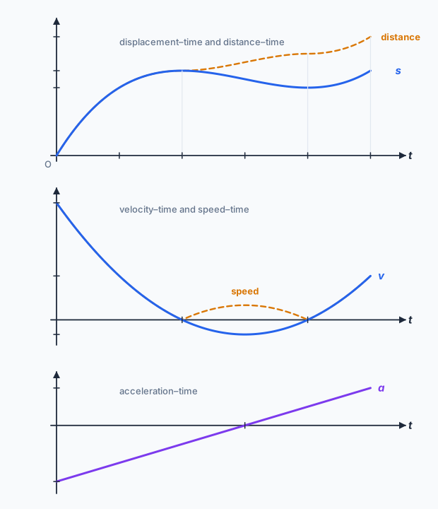
Displacement is where the particle is relative to \(O\). Distance is how far it has gone. They differ as soon as the particle turns round. To find the distance travelled over an interval: find every time the particle is at rest inside it, work out \(s\) at the start, at each turning time and at the end, and add up the sizes of the changes.
Reading the graphs
- The gradient of a displacement–time graph is velocity; of a velocity–time graph, acceleration.
- The area under a velocity–time graph is displacement (area below the axis counts negative); under a speed–time graph it is distance.
- The speed–time graph is the velocity–time graph with the negative parts reflected, exactly like \( y = |f(x)| \) in Topic 1; distance–time never decreases.
✏️Worked example 1 (no calculator)
(a) \( v = 3t^{2} - 18t + 24 = 3(t - 2)(t - 4) \), so the particle is at rest at \( t = 2 \) and \( t = 4 \).
(b) \( a = 6t - 18 \), so \( a = -12 \) m s−2 at \( t = 1 \). (The particle is still moving forwards, but slowing down.)
(c) \( s(0) = 0 \), \( s(2) = 20 \), \( s(4) = 16 \), \( s(5) = 20 \). The particle goes out 20 m, comes back 4 m, then goes forward 4 m again:
✏️Worked example 2 (calculator)
(a) \( a = \dfrac{dv}{dt} = 4e^{-0.5t} \); at \( t = 2 \), \( a = 4e^{-1} = 1.47 \) m s−2.
(b) \( s = \int (8 - 8e^{-0.5t})\,dt = 8t + 16e^{-0.5t} + c \). At \( t = 0 \), \( s = 0 \): \( 0 = 16 + c \), so \( c = -16 \). At \( t = 4 \): \( s = 32 + 16e^{-2} - 16 = 18.2 \) m.
(c) \( e^{-0.5t} \to 0 \), so \( v \to 8 \) m s−1. Since \( v > 0 \) for all \( t > 0 \), the particle never turns round, and here the distance equals the displacement.
📝Practise
Written in the style of the current Paper 1 (no calculator) and Paper 2 (calculator) questions.
1. (No calculator.) A particle has velocity \( v = 2t^{2} - 14t + 20 \) m s−1. Find the times when it is at rest, and its acceleration when \( t = 1 \). [4]
2. (No calculator.) A particle passes \(O\) at \( t = 0 \) with velocity 3 m s−1, and its acceleration is \( a = 6t - 4 \). (a) Find \(v\) and \(s\) in terms of \(t\). (b) Show that the particle is never at rest. [6]
3. (No calculator.) A particle moves so that \( s = 2\sin 3t \) m. Find the first time after \( t = 0 \) at which it is at rest, and its acceleration at that time. [4]
4. (Calculator.) A particle has velocity \( v = 5e^{-0.2t} \) m s−1. Find its initial acceleration and the distance travelled in the first 10 seconds. [5]
5. (Calculator.) A particle has velocity \( v = t^{2} - 6t + 8 \) m s−1 for \( 0 \le t \le 5 \). Find the total distance travelled and the final displacement from the starting point. [6]
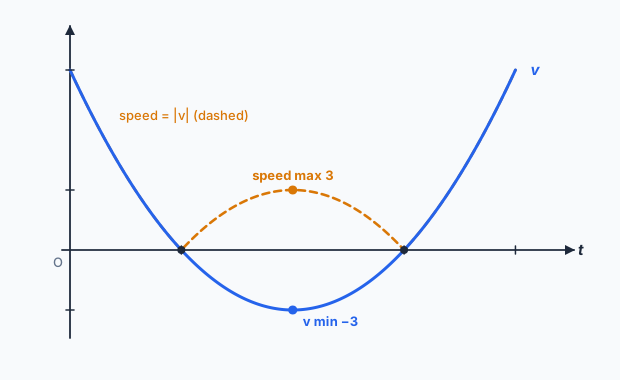
6. (No calculator.) For \( v = 3(t - 1)(t - 3) \), \( 0 \le t \le 4 \), describe the velocity–time and speed–time graphs, giving the key values. [4]
🔗Go deeper — other people’s work
These are external resources, not mine. If one stops working, tell me and everything above it on this page still stands.
- Desmos — plot \(s\), \(v\) and \(a\) on the same axes to see how the zeros of one line up with the turning points of another
- PhET “The Moving Man” — drag a figure and watch position, velocity and acceleration graphs draw themselves