Concluding and evaluating
🎯What you need to be able to do
- State a conclusion that answers the research question, supported by the data.
- Compare a result with an accepted value using the uncertainty, not the percentage difference alone.
- Say what the gradient and intercept of your graph physically mean.
- Distinguish the effect of random error from that of systematic error on your result.
- Identify methodological weaknesses and rank them by how much they mattered.
- Propose realistic improvements, each addressing a named weakness.
- Suggest a sensible extension to the investigation.
✅Writing a conclusion
A conclusion answers the research question — in a sentence, using the data. Everything else in it is support for that sentence. Three things belong there:
Say what the gradient and intercept actually mean. A gradient of 4.02 s² m−1 is not a conclusion; “the gradient is \( 4\pi^{2}/g \), giving \( g = 9.8 \pm 0.6 \) m s−2” is. And an intercept that theory says should be zero is worth a sentence whether it was zero or not.
⚖️Comparing with an accepted value
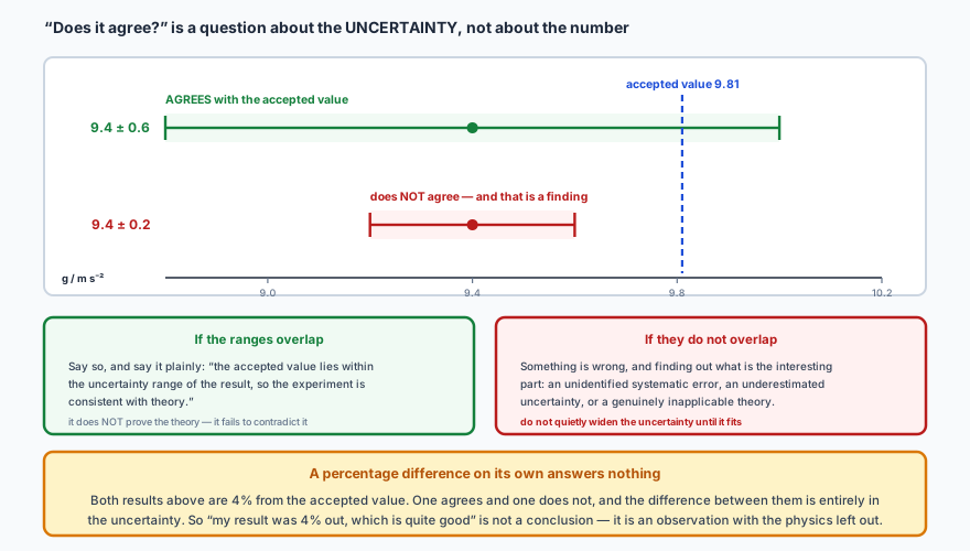
So the question is never “how close was I?” but “does the accepted value lie inside my uncertainty range?” If it does, the experiment is consistent with theory. If it does not, that is a real result and worth chasing: it means an unidentified systematic error, an underestimated uncertainty, or a theory that does not apply in your conditions.
🔍What each kind of error did
The evaluation has to distinguish two quite different things, because they have different fixes and they show up differently in the data.
That second one is the useful diagnostic. If your graph should pass through the origin and does not, you have measured a systematic error rather than merely suspected one — and its size is the intercept. A zero error on an instrument, a background count, a lead resistance, all announce themselves this way.
✏️Worked example 1 — a conclusion, written out
The relationship. The graph of \( T^{2} \) against \(l\) is a straight line, so \( T^{2} \propto l \) and therefore \( T \propto \sqrt{l} \), as theory predicts.
What the gradient gives. Theory says the gradient is \( 4\pi^{2}/g \):
The comparison. The accepted value of 9.81 m s−2 lies well inside that range, so the result is consistent with theory.
The intercept. Theory predicts zero, and the measured intercept is \( 0.05 \pm 0.08 \) s² — which includes zero. So there is no evidence of a systematic error in the length or timing measurements, and saying so is part of the conclusion.
🔧Weaknesses and improvements
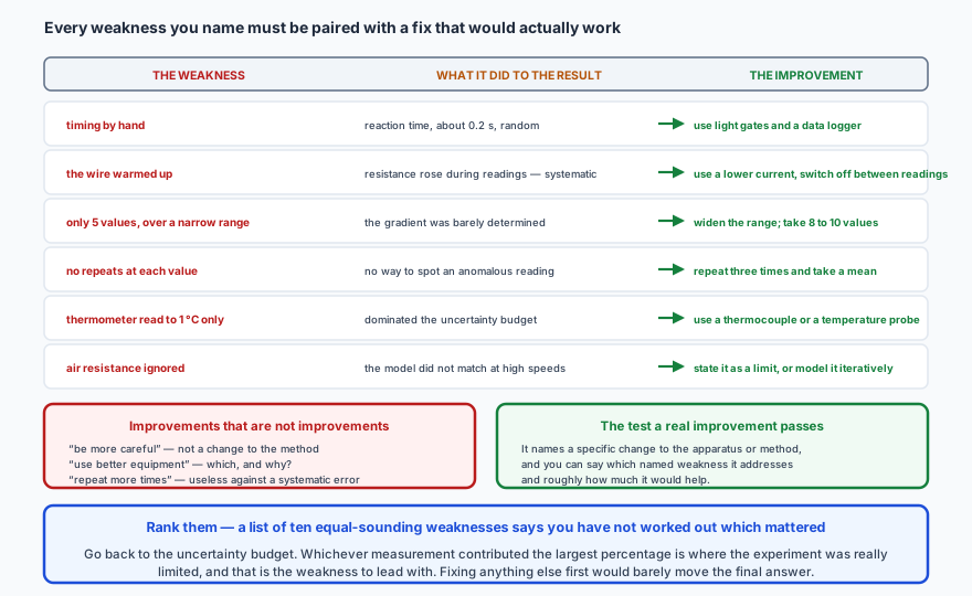
The single most useful thing an evaluation can do is rank the weaknesses. Go back to the uncertainty budget: whichever measurement contributed the largest percentage is where the experiment was really limited, and that is the one to lead with. A list of ten equal-sounding problems says you have not worked out which mattered.
✏️Worked example 2 — diagnosing a disagreement
Does it agree? The range is \( 5.5 \) to \( 6.1 \times 10^{-7} \), and 4.9 is outside it. So no — and the disagreement is substantial, roughly three times the quoted uncertainty.
Which way is it wrong? The measured resistivity is too high. Since \( \rho = RA/l \), that means either \(R\) came out too high, \(A\) too high, or \(l\) too low.
The intercept is the clue. A graph of \(R\) against \(l\) should pass through the origin: zero length, zero resistance. An intercept of \( +0.42\ \Omega \) says every resistance reading was about \( 0.42\ \Omega \) too high — almost certainly the resistance of the leads and the crocodile clips, in series with the wire in every measurement.
Does that explain the size of the discrepancy? If the wire resistances were of order a few ohms, an extra \( 0.42\ \Omega \) on each is a substantial systematic addition — in the right direction, and plausibly of the right size.
➡️Extending the investigation
A good extension asks the next question rather than repeating this one more carefully. It usually comes from one of three places: a variable you held constant that could now be varied; a range you could not reach with the apparatus available; or an assumption the analysis relied on that could be tested directly.
📝Practise
Work through these, then reveal the answer. Each question targets a different objective from the list above.
1. A student concludes: “My value for \(g\) was 9.4 m s−2, which is 4% from the accepted value, so the experiment was quite successful.” Explain what is missing.
If the result were \( 9.4 \pm 0.6 \) m s−2, then 9.81 lies inside the range and the experiment is consistent with theory. If it were \( 9.4 \pm 0.2 \), then 9.81 lies outside and something is wrong — despite being the same 4% away.
“Quite successful” is also doing no work: the conclusion should state whether the result is consistent with theory and, if not, what that suggests.
2. A result is \( 2.6 \pm 0.2 \) and the accepted value is \( 3.1 \). State whether it agrees, and describe the two possibilities.
Two possibilities, and they need different responses:
An unidentified systematic error. Something shifted every reading in the same direction — a zero error, a miscalibrated instrument, a consistently flawed technique, or a quantity that was not held constant. Look for an unexpected intercept on the graph.
An underestimated uncertainty. The true uncertainty may be larger than ± 0.2 — perhaps a source of error was not included in the budget at all. That is a genuine possibility, but it must be argued from evidence, not assumed because it would be convenient.
3. Explain how random error and systematic error each show up differently on a graph.
Systematic error does not scatter the points at all — it shifts them. It typically shows up as an unexpected intercept: a graph that theory says should pass through the origin but does not. It can also appear as a gradient that is consistently wrong, if the error scales with the measurement rather than being a fixed offset.
The practical consequence: scattered points around a line through the origin means poor precision but no obvious systematic problem, while tightly grouped points on a line with an unexplained intercept means the opposite.
4. A graph of extension against load should pass through the origin but has an intercept of −0.4 cm. Suggest a cause and a correction.
That is a systematic error: every extension carries the same offset.
Correction: add 0.4 cm to every extension, or better, use the gradient to find the spring constant. A constant offset shifts the intercept but not the gradient, so \(k\) obtained from the gradient is unaffected by this error — which is one of the main reasons for plotting a graph rather than calculating from single readings.
5. Explain why “human error” and “be more careful” are not acceptable in an evaluation.
“Be more careful” is not a change to the method: the same apparatus, operated by the same person with the same technique, will produce the same uncertainty however much resolve is applied.
A usable weakness names what went wrong, which direction it pushed the result and roughly how much; a usable improvement names a specific change — “replace hand timing with light gates, removing the ± 0.2 s reaction-time uncertainty”.
6. Why is “take more repeats” a poor improvement when the dominant error is systematic?
Taking a hundred readings with a micrometer that has a − 0.03 mm zero error gives a beautifully precise answer that is still 0.03 mm wrong. The extra effort improves the precision, does nothing for the accuracy, and may even be counter-productive if it creates false confidence.
The fix for a systematic error is to find its cause and correct for it — measure the zero error and subtract it, measure the lead resistance and subtract it, subtract the background count.
7. Given an uncertainty budget of: length 0.2%, diameter 5.2%, current 4%, potential difference 0.7% — state which weakness to lead with and what to propose.
Proposals, in order of usefulness: measure the diameter at more points along the wire and average, since the wire may not be perfectly uniform; use a thicker wire, so the same ± 0.01 mm micrometer uncertainty is a smaller percentage; or use a micrometer with a finer resolution if one is available.
Note what not to lead with: improving the length measurement from 0.2% would be invisible in the final answer, and proposing it first suggests the budget was never examined.
8. Distinguish a weakness from a limitation, and give an example of each.
A limitation is a constraint on what the investigation could establish at all, given the apparatus, the time or the physics. Example: the conclusion applies only to amplitudes below about 15°, because the small-angle approximation underpins the theory being tested, and larger amplitudes were not investigated.
Both belong in an evaluation, and they lead to different things: a weakness leads to an improvement, a limitation leads to an extension.
9. An investigation into how the resistance of a wire depends on its length is complete. Suggest two genuine extensions and say where each came from.
From an assumption: the analysis assumed the wire's temperature stayed constant, which is why the current was kept low. Test it directly — investigate how the resistance depends on temperature, using a water bath over a controlled range.
Both ask a new question rather than repeating the old one more carefully, which is what makes them extensions rather than improvements.
10. Write a two-sentence conclusion for an experiment whose \( T^{2} \) against \(l\) graph gave a gradient of \( 4.15 \pm 0.30 \) s² m−1 and an intercept of \( 0.02 \pm 0.06 \) s².
“The graph of \( T^{2} \) against \(l\) is a straight line, confirming that \( T \propto \sqrt{l} \); its gradient of \( 4.15 \pm 0.30 \) s² m−1 corresponds to \( g = 9.5 \pm 0.7 \) m s−2, and the accepted value of 9.81 m s−2 lies within that range, so the result is consistent with theory. The intercept of \( 0.02 \pm 0.06 \) s² includes zero, as theory requires, giving no evidence of a systematic error in the timing or length measurements.”
Both sentences do work: the first answers the research question and compares with theory, the second interprets the intercept — which most reports omit entirely.
🔗Go deeper — other people’s work
These are external resources, not mine. If one stops working, tell me and everything above it on this page still stands.
- The IB Physics guide internal assessment criteria — conclusion and evaluation are a third of the marks
- NIST reference values — for the accepted figures your result should be compared against