HomeLearning HubIB DP PhysicsT.3 Mathematics
T.3

Mathematics

Tools and inquiry · skills assessed across the whole course

The longest page in this section, because it carries the machinery every other topic borrows: units, vectors, uncertainties and graphs. None of it is difficult. All of it is where marks quietly disappear.

🎯What you need to be able to do

  • Name the SI base units, express a derived unit in base units, and use prefixes correctly.
  • Estimate to an order of magnitude, and use scientific notation and significant figures properly.
  • Check an equation by dimensional analysis, using SI base units.
  • Distinguish vectors from scalars, resolve a vector into components, and add vectors.
  • Distinguish random from systematic error, and precision from accuracy.
  • Estimate an uncertainty from an instrument and from a set of repeats, and quote it properly.
  • Combine uncertainties through addition, multiplication, division and powers.
  • Read a gradient, intercept and area from a graph, and say what each represents.
  • Choose what to plot to linearise a relationship, including using logarithms.
  • Draw error bars, and find the uncertainty in a gradient and an intercept from them.

📏Units, and the seven everything is built from

A measurement is a number and a unit; without both it says nothing. Seven base units are defined outright, and every other unit in physics is a derived unit — some combination of those seven, occasionally given a name of its own.
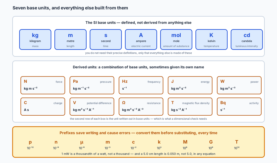
The seven SI base units shown as cards: the kilogram for mass, metre for length, second for time, ampere for electric current, mole for amount of substance, kelvin for temperature and candela for luminous intensity, with a note that their precise definitions are not needed, only that everything else is made from them. Below, ten derived units each with its symbol, what it measures and its expression in base units: the newton as kilogram metre per second squared, the pascal, hertz, joule, watt, coulomb as ampere second, volt, ohm, tesla and becquerel. A footer strip lists the prefixes from pico at ten to the minus twelve through nano, micro, milli, centi, kilo, mega, giga to tera at ten to the twelve, warning that one milliwatt is a thousandth of a watt and that a 5.0 centimetre length is 0.050 metres in any equation.
The base-unit column is the one that earns marks. It is what a dimensional check needs, and it is how you work out what a gradient or an area on a graph physically represents.

The commonest unit error is not exotic: it is failing to convert a prefix before substituting. A length of 5.0 cm goes into an equation as 0.050 m, and a current of 250 mA as 0.250 A. Convert everything to base units first, and the answer comes out in base units automatically.

🔢Orders of magnitude, notation and significant figures

Physics spans a preposterous range, from \( 10^{-30} \) kg to \( 10^{53} \) kg, and the only way to hold that in your head is to work in orders of magnitude — the nearest power of ten. Ratios then become subtractions of exponents, which you can do in your head.
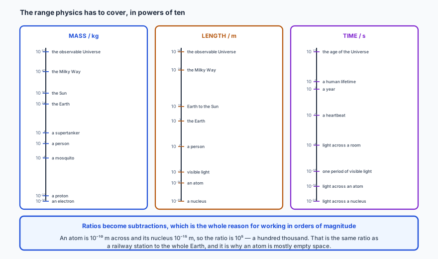
Three vertical logarithmic scales. Mass in kilograms runs from ten to the fifty-three for the observable Universe, through ten to the forty-two for the Milky Way, ten to the thirty for the Sun, ten to the twenty-four for the Earth, ten to the eight for a supertanker, ten squared for a person and ten to the minus six for a mosquito, down to ten to the minus twenty-seven for a proton and minus thirty for an electron. Length in metres runs from ten to the twenty-six for the observable Universe down to ten to the minus fifteen for a nucleus, passing an atom at minus ten and visible light at minus seven. Time in seconds runs from ten to the seventeen for the age of the Universe down to ten to the minus twenty-three for light to cross a nucleus. A note explains that an atom is ten to the minus ten metres across and its nucleus ten to the minus fifteen, a ratio of a hundred thousand, the same ratio as a railway station to the whole Earth.
Worth developing a feel for rather than memorising. The value of it is catching a calculator slip: if an answer for the mass of a molecule comes out at \( 10^{-3} \) kg, something went in wrong.

Scientific notation writes any number as \( a \times 10^{b} \) with \( 1 \le a < 10 \). Significant figures then carry an implied uncertainty: quoting 23.456 g claims five significant figures and so an uncertainty around ± 0.001 g, while 23.5 g claims three and implies ± 0.1 g. When multiplying or dividing, quote the answer to the fewest significant figures of any input — \( 4.2 \times 3.14159 = 13.194678 \) on a calculator, but 4.2 has only two significant figures, so the answer is 13.

The trap: a calculator's digits are not significant figures. Copying out 13.194678 when one of your measurements was good to two figures claims a precision a thousand times better than you had. It is not a rounding nicety — it is a false claim about the experiment, and it is marked as one. The same applies to an uncertainty: round it to one significant figure first, then round the value to match its decimal place.

⚖️Dimensional analysis

Every term in a physically correct equation must have the same units. That gives you a free check on any equation you are unsure of: write each term in SI base units and see whether they match.

check \( s = ut + \tfrac{1}{2}at^{2} \)m = (m s−1)(s) = (m s−2)(s2) — all metres
so the equationis dimensionally possible

Two limits are worth knowing. First, pure numbers have no units, so the \( \tfrac{1}{2} \) above is invisible to the check — which means dimensional analysis can tell you an equation is wrong, but never that it is right. The equation \( s = 3at^{2} \) passes the same check and is still false. Second, it says nothing about whether you have the physics the right way round.

✏️Worked example 1 — catching a wrong formula with units

A student writes the period of a mass on a spring as \( T = 2\pi\sqrt{m/k^{2}} \), where \(k\) is the spring constant. Show by dimensional analysis that this cannot be right, and find the correct form.

Get every quantity into base units. The spring constant is force per unit extension:

\[ k = \frac{\text{N}}{\text{m}} = \frac{\text{kg m s}^{-2}}{\text{m}} = \text{kg s}^{-2} \]

Test the student's version. The left-hand side is a time, so it must come out in seconds:

\[ \sqrt{\frac{\text{kg}}{(\text{kg s}^{-2})^{2}}} = \sqrt{\frac{\text{kg}}{\text{kg}^{2}\,\text{s}^{-4}}} = \sqrt{\text{kg}^{-1}\text{s}^{4}} = \text{kg}^{-1/2}\,\text{s}^{2} \]

That is not seconds, so the formula is wrong.

Try it without the square on \(k\).

\[ \sqrt{\frac{\text{kg}}{\text{kg s}^{-2}}} = \sqrt{\text{s}^{2}} = \text{s} \quad \checkmark \]
\[ T = 2\pi\sqrt{\frac{m}{k}} \]
Sanity check. The units now balance, and the \( 2\pi \) is a pure number so it cannot upset them. Note what this method did and did not do: it ruled the first version out with certainty, and it confirmed the second is possible — but a formula \( T = 5\sqrt{m/k} \) would pass the identical check. Dimensional analysis is a filter, not a proof.

Vectors and scalars

A scalar has magnitude only; a vector has magnitude and direction. The distinction matters because it changes the arithmetic: two 3 N and 4 N forces total 7 N only if they point the same way, and can total anything down to 1 N if they do not.
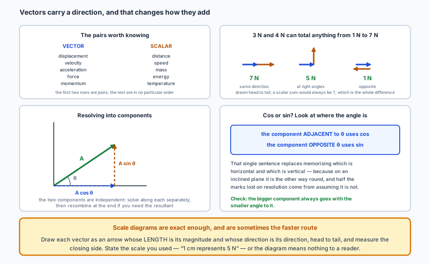
Four panels. First, a list pairing vectors with scalars: displacement with distance, velocity with speed, and then acceleration, force and momentum against mass, energy and temperature. Second, three additions of a 3 newton and a 4 newton force drawn head to tail, giving 7 newtons in the same direction, 5 newtons at right angles and 1 newton opposite, with a note that a scalar sum would always be 7. Third, a vector A resolved into components, with A cos theta along the axis adjacent to the angle and A sin theta opposite it, and a note that the two components are independent so each can be solved separately. Fourth, the rule for choosing between cosine and sine: the component adjacent to theta uses cos and the component opposite theta uses sin, with the check that the bigger component always goes with the smaller angle to it.
“Adjacent uses cos, opposite uses sin” is worth more than memorising that horizontal is cosine — on an inclined plane it is the other way round, and that is where the marks go.

Resolving splits a vector into two perpendicular components, and those components are completely independent: you can solve along one without reference to the other and recombine at the end. That is the single most useful technique in mechanics.

🎯Random and systematic error

Two words that get used loosely and mean quite different things. Precision is about how closely repeated readings agree with each other; accuracy is about how close they are to the true value. An experiment can have either without the other.
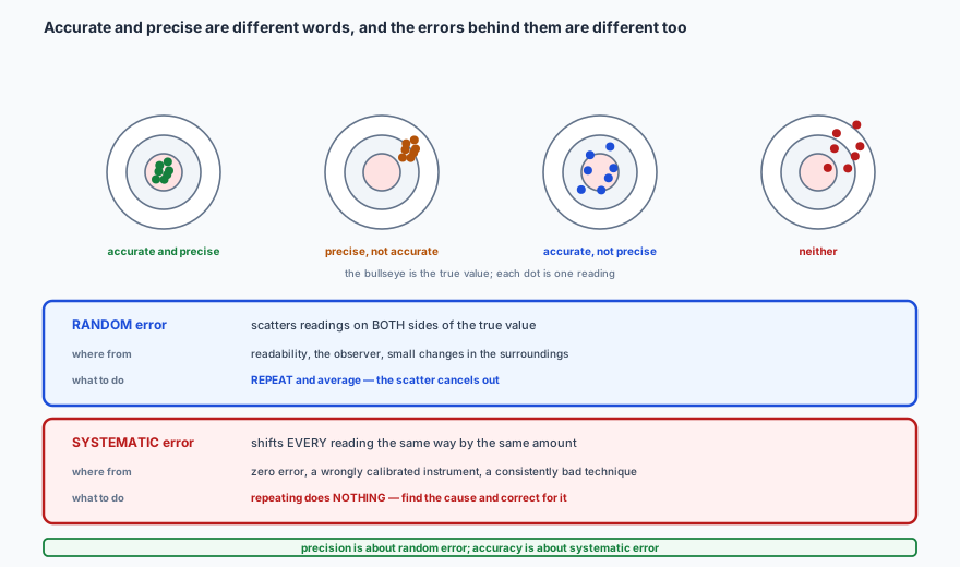
Four targets showing readings as dots against a bullseye representing the true value. In the first the dots are tightly clustered on the bullseye and it is labelled accurate and precise. In the second they are tightly clustered but off to one side, labelled precise but not accurate. In the third they are widely scattered but centred on the bullseye, labelled accurate but not precise. In the fourth they are widely scattered and off centre, labelled neither. Two panels follow. Random error scatters readings on both sides of the true value, comes from readability, the observer and small changes in the surroundings, and is dealt with by repeating and averaging so the scatter cancels. Systematic error shifts every reading the same way by the same amount, comes from a zero error, a wrongly calibrated instrument or a consistently bad technique, and repeating does nothing about it.
The second target is the dangerous one: tightly grouped readings look convincing, and a systematic error will keep them tightly grouped in the wrong place all day.
random erroraffects PRECISION — reduce it by repeating and averaging
systematic erroraffects ACCURACY — repeating will never reveal it

📐Getting an uncertainty in the first place
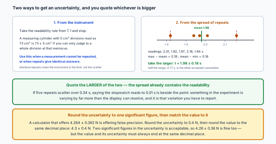
Two routes to an uncertainty. The first is from the instrument, applying the readability rule, so a measuring cylinder with 5 cubic centimetre divisions read as 73 gives 73 plus or minus 5, and this route is used when a measurement cannot be repeated or when repeats give identical answers. The second is from the spread of repeats: five timings of 2.01, 1.82, 1.97, 2.16 and 1.94 seconds are plotted on a number line with their mean of 1.98 marked, and since the largest reading is 0.18 above the mean while the smallest is 0.16 below, the larger gap is taken and the result quoted as 1.98 plus or minus 0.18 seconds. Notes add that half the range, 0.17, is the other accepted convention, that the larger of the two routes should be quoted, and that the uncertainty should be rounded to one significant figure with the value matched to the same decimal place.
If five repeats scatter over a third of a second, the fact that the stopwatch displays hundredths is beside the point. Something in the experiment is varying by more than the instrument can resolve, and that variation is what you report.

Combining uncertainties

Three rules cover nearly everything, and picking the right one is entirely a matter of looking at what the formula does to the quantities.
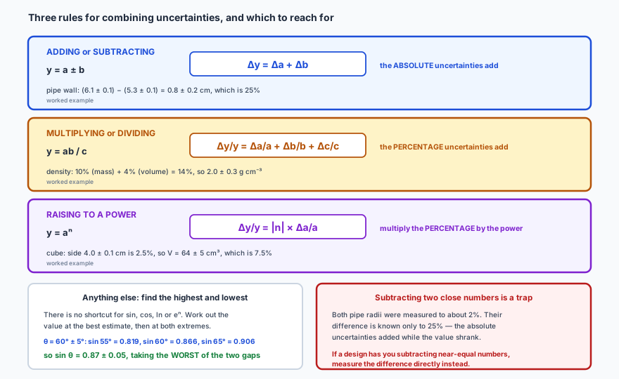
Three rules set out in rows. For adding or subtracting, y equals a plus or minus b, the absolute uncertainties add, worked through a pipe wall where 6.1 plus or minus 0.1 minus 5.3 plus or minus 0.1 gives 0.8 plus or minus 0.2 centimetres, which is 25 per cent. For multiplying or dividing, y equals a b over c, the percentage uncertainties add, worked through a density where 10 per cent from the mass plus 4 per cent from the volume gives 14 per cent, so 2.0 plus or minus 0.3 grams per cubic centimetre. For raising to a power, y equals a to the n, the percentage is multiplied by the power, worked through a cube whose side of 4.0 plus or minus 0.1 centimetres is 2.5 per cent, giving a volume of 64 plus or minus 5 cubic centimetres, or 7.5 per cent. Two further panels cover functions with no shortcut, where sine of 60 plus or minus 5 degrees is evaluated at all three angles to give 0.87 plus or minus 0.05, and a warning that subtracting two close numbers is a trap.
Notice the pattern: absolute uncertainties add when you add or subtract, percentage uncertainties add when you multiply or divide. Mixing the two up is the most common error on this topic.

✏️Worked example 2 — density, both ways

A block has a mass of 10 ± 1 g and a volume of 5.0 ± 0.2 cm³. Find its density with its uncertainty, first by finding the largest and smallest possible values, then by the percentage shortcut.

Best value. \( \rho = m/V = 10/5.0 = 2.0 \) g cm−3.

The full range. Density is largest when the mass is at its largest and the volume at its smallest — note that they go opposite ways, because \(V\) is on the bottom:

\[ \rho_{\text{max}} = \frac{11}{4.8} = 2.29, \qquad \rho_{\text{min}} = \frac{9}{5.2} = 1.73 \]

Both are about 0.3 away from 2.0, so \( \rho = 2.0 \pm 0.3 \) g cm−3.

The shortcut. Division, so the percentage uncertainties add:

\[ \frac{1}{10} = 10\%, \qquad \frac{0.2}{5.0} = 4\%, \qquad 10 + 4 = 14\% \]
\[ 14\% \text{ of } 2.0 = 0.28 \approx 0.3 \]
Sanity check. The two routes agree exactly, which is the whole reason the shortcut is allowed. Use the shortcut in practice — it is faster and less error-prone — but knowing where it comes from is what lets you handle the cases it does not cover, like the sine in the previous figure. Note also the rounding: 0.28 becomes 0.3, one significant figure, and the value is then quoted to the matching decimal place.
The trap: subtracting two nearly equal numbers destroys precision. Two pipe radii each measured to about 2% give a wall thickness known only to 25%, because the absolute uncertainties added while the value itself shrank to almost nothing. If an experimental design has you subtracting two similar measurements, look for a way to measure the difference directly instead — and if you cannot, say in the evaluation that this is where the precision went.

📈Reading a graph

A graph gives you three things the raw table does not: an intercept, a gradient and an area. What each one means physically you can always work out from the axis units.
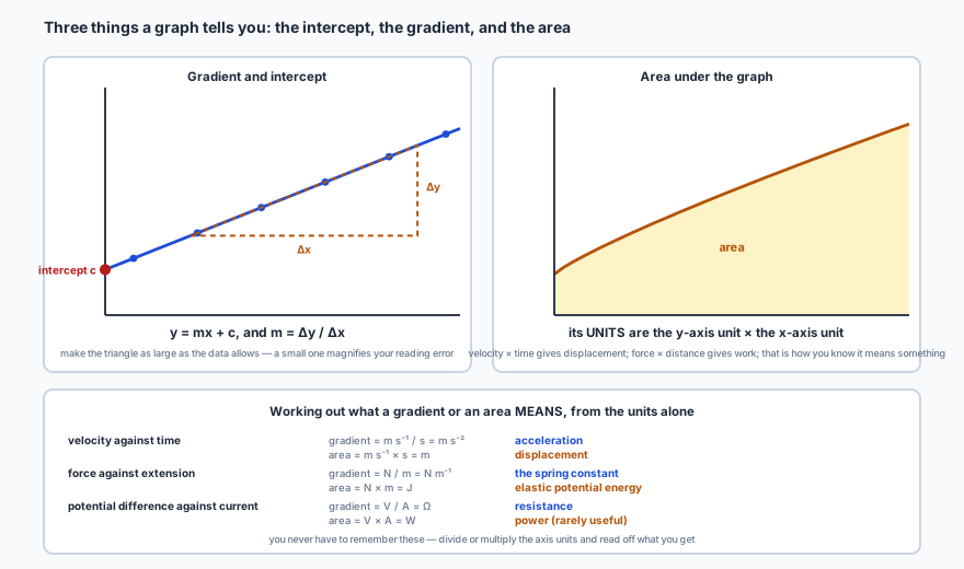
On the left, a straight-line graph with its y-intercept marked and a large dashed gradient triangle spanning most of the data, labelled delta x along the base and delta y up the side, with the relations y equals m x plus c and m equals delta y over delta x, and advice to make the triangle as large as the data allows because a small one magnifies reading error. On the right, a curve with the area beneath it shaded, noting that the units of the area are the y-axis unit multiplied by the x-axis unit. A table then works out what gradients and areas mean for three common graphs: for velocity against time the gradient is acceleration and the area is displacement; for force against extension the gradient is the spring constant and the area is elastic potential energy; for potential difference against current the gradient is resistance.
You never have to remember what a gradient represents. Divide the y-axis unit by the x-axis unit and read off what you get — m s−1 over s is m s−2, which is an acceleration.

📏Choosing what to plot

A straight line is worth far more than a curve: you can judge it by eye, its gradient uses every point at once, and a systematic error shows up as an unexpected intercept. So the standard move is to rearrange the physics into the form \( y = mx + c \) and plot whatever that requires.
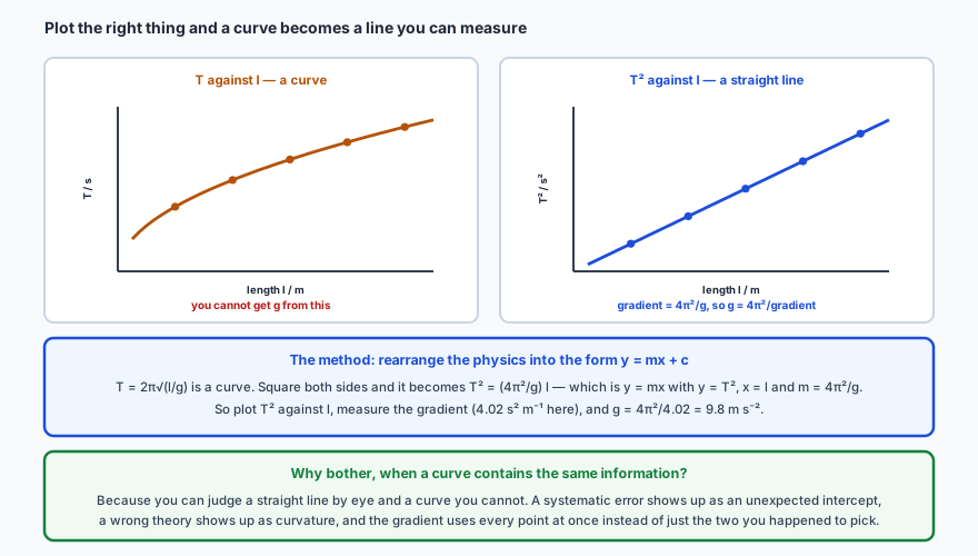
Two graphs of the same pendulum data. On the left, the period T plotted against length l gives a curve from which the acceleration of free fall cannot be extracted. On the right, T squared plotted against l gives a straight line through the origin whose gradient is four pi squared over g, so g equals four pi squared divided by the gradient. A panel explains the method: T equals two pi root l over g is a curve, but squaring both sides gives T squared equals four pi squared over g times l, which is y equals m x with y as T squared, x as l and m as four pi squared over g, so measuring the gradient of 4.02 square seconds per metre gives g as 9.8 metres per second squared. A second panel explains why this is worth doing: a straight line can be judged by eye, a systematic error shows up as an unexpected intercept, a wrong theory shows up as curvature, and the gradient uses every point rather than two.
Both graphs contain identical information. Only one of them lets you get \(g\) by drawing a line with a ruler.

HLTwo shapes resist that treatment, and both yield to logarithms.
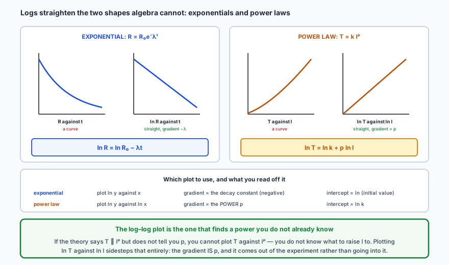
On the left, an exponential relationship R equals R nought e to the minus lambda t: plotted directly it is a curve, but plotting the natural log of R against t gives a straight line of gradient minus lambda, because ln R equals ln R nought minus lambda t. On the right, a power law T equals k l to the p: plotted directly it is a curve, but plotting ln T against ln l gives a straight line whose gradient is the power p, because ln T equals ln k plus p ln l. A table summarises which plot to use and what to read off: for an exponential plot ln y against x, the gradient is the decay constant and the intercept is the log of the initial value; for a power law plot ln y against ln x, the gradient is the power and the intercept is the log of k. A closing note explains that the log-log plot is the one that finds a power you do not already know.
HLThe log–log plot has a property nothing else does: it finds the power experimentally. If theory says \( T \propto l^{p} \) but not what \(p\) is, you cannot plot \(T\) against \( l^{p} \) — but the gradient of \( \ln T \) against \( \ln l \) simply is \(p\).

Error bars, and the uncertainty in a gradient
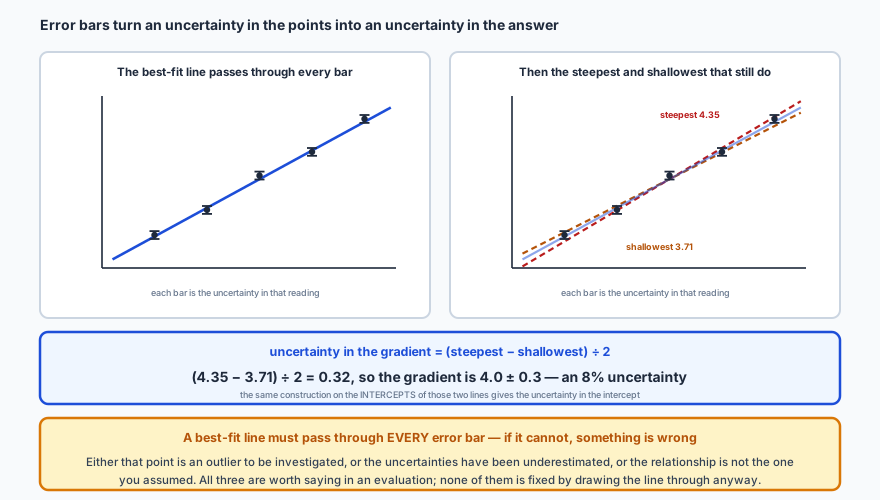
Two plots of the same five data points, each drawn with a vertical error bar. On the left a single best-fit line is drawn which passes through every error bar. On the right, two further lines are added: the steepest line that still passes through all the bars, with a gradient of 4.35, and the shallowest, with a gradient of 3.71, both pivoting about the middle of the data. The uncertainty in the gradient is then half the difference between them, so 4.35 minus 3.71 over 2 gives 0.32 and the gradient is 4.0 plus or minus 0.3, an 8 per cent uncertainty, with the same construction on the intercepts giving the uncertainty in the intercept. A closing note warns that a best-fit line must pass through every error bar, and that if it cannot then either the point is an outlier, the uncertainties were underestimated, or the relationship is not the one assumed.
This is how an uncertainty in your readings becomes an uncertainty in your final answer — and it is the step most often left out of an investigation that has done everything else properly.
\[ \text{uncertainty in gradient} = \frac{m_{\text{steepest}} - m_{\text{shallowest}}}{2} \]

✏️Worked example 3 — from a graph to a value of \(g\), with its uncertainty

A pendulum experiment gives a graph of \( T^{2} \) against \(l\). The best-fit gradient is 4.02 s² m−1; the steepest and shallowest lines consistent with the error bars have gradients 4.28 and 3.76. Find \(g\) and its uncertainty.

The relationship. \( T = 2\pi\sqrt{l/g} \) squares to \( T^{2} = (4\pi^{2}/g)\,l \), so the gradient is \( 4\pi^{2}/g \) and

\[ g = \frac{4\pi^{2}}{\text{gradient}} = \frac{39.48}{4.02} = 9.82\ \text{m s}^{-2} \]

Uncertainty in the gradient.

\[ \Delta m = \frac{4.28 - 3.76}{2} = 0.26\ \text{s}^{2}\,\text{m}^{-1}, \qquad \frac{0.26}{4.02} = 6.5\% \]

Carry it through. \(g\) is \( 4\pi^{2} \) divided by the gradient, and \( 4\pi^{2} \) is a pure number with no uncertainty. Dividing by a quantity passes its percentage uncertainty straight through:

\[ \frac{\Delta g}{g} = 6.5\%, \qquad \Delta g = 0.065 \times 9.82 = 0.64\ \text{m s}^{-2} \]
\[ g = 9.8 \pm 0.6\ \text{m s}^{-2} \]
Sanity check. The accepted 9.81 m s−2 lies comfortably inside \( 9.8 \pm 0.6 \), so the experiment agrees with theory — and saying that, rather than just quoting the number, is what a conclusion is for. Note the rounding: the uncertainty goes to one significant figure (0.6) and the value is then given to the matching decimal place (9.8), not the 9.82 the calculator offered.

📝Practise

Work through these, then reveal the answer. Each question targets a different objective from the list above.

1. Express the volt in SI base units, starting from the definition of potential difference as energy per unit charge.
Potential difference is energy per unit charge, so \( \text{V} = \text{J}/\text{C} \).
Energy is force × distance: \( \text{J} = \text{N m} = (\text{kg m s}^{-2})(\text{m}) = \text{kg m}^{2}\,\text{s}^{-2} \).
Charge is current × time: \( \text{C} = \text{A s} \).
So \[ \text{V} = \frac{\text{kg m}^{2}\,\text{s}^{-2}}{\text{A s}} = \text{kg m}^{2}\,\text{s}^{-3}\,\text{A}^{-1} \] The method is always the same: break each named unit down until only the seven base units are left.
2. Convert to SI base units: (a) 250 mA; (b) 5.0 cm; (c) 2.5 GHz; (d) 40 µC.
(a) \( 250 \times 10^{-3} = 0.250 \) A.
(b) \( 5.0 \times 10^{-2} = 0.050 \) m.
(c) \( 2.5 \times 10^{9} \) Hz, which in base units is \( 2.5 \times 10^{9}\ \text{s}^{-1} \).
(d) \( 40 \times 10^{-6} = 4.0 \times 10^{-5} \) C.
Do this conversion before substituting into any equation, not after. Working in centimetres and then wondering why an answer is out by a factor of a hundred is the single most common arithmetic failure in the subject.
3. A student suggests that the drag force on a sphere is \( F = 6\pi\eta rv \), where \( \eta \) has base units kg m−1 s−1, \(r\) is a radius and \(v\) a speed. Check this by dimensional analysis.
Work out the base units of the right-hand side. The \( 6\pi \) is a pure number and has none: \[ (\text{kg m}^{-1}\text{s}^{-1})(\text{m})(\text{m s}^{-1}) = \text{kg m}^{-1+1+1}\,\text{s}^{-1-1} = \text{kg m s}^{-2} \] The left-hand side is a force, and a newton is \( \text{kg m s}^{-2} \). They match, so the equation is dimensionally possible.
Note the limit of the check: it confirms the equation could be right. \( F = 20\pi\eta rv \) would pass the identical test, because a dimensionless constant is invisible to this method.
4. A force of 25 N acts at 40° above the horizontal. Find its horizontal and vertical components, and check your answer without a calculator.
The horizontal component is adjacent to the 40° angle, so it uses cosine; the vertical is opposite, so it uses sine. \[ F_H = 25\cos 40^\circ = 19.2\ \text{N}, \qquad F_V = 25\sin 40^\circ = 16.1\ \text{N} \] Check without a calculator: 40° is less than 45°, so the component nearer the angle — the horizontal one — must be the larger. It is. Also, both components must be smaller than the 25 N resultant, and \( \sqrt{19.2^2 + 16.1^2} = 25.1 \approx 25 \) N recovers it.
5. Explain the difference between a random and a systematic error, and state what each does to precision and accuracy. Give one example of each.
A random error scatters readings on both sides of the true value, in an unpredictable way. It comes from the readability of the instrument, from the observer, or from small uncontrolled changes in the surroundings. It reduces precision, and repeating the measurement and averaging reduces it, because the scatter tends to cancel. Example: reading a stopwatch by hand.

A systematic error shifts every reading in the same direction by the same amount. It comes from a zero error, a wrongly calibrated instrument, or a consistently flawed technique. It reduces accuracy, and repeating does nothing about it — the mean is displaced by exactly the same amount as each reading. Example: a micrometer that reads −0.03 mm when closed.
6. A block has a mass of 24.0 ± 0.5 g and a volume of 3.0 ± 0.1 cm³. Find its density with its uncertainty.
Best value: \( \rho = 24.0/3.0 = 8.0 \) g cm−3.
This is a division, so the percentage uncertainties add: \[ \frac{0.5}{24.0} = 2.1\%, \qquad \frac{0.1}{3.0} = 3.3\%, \qquad \text{total } 5.4\% \] \[ 5.4\% \text{ of } 8.0 = 0.43 \approx 0.4 \] So \( \rho = 8.0 \pm 0.4 \) g cm−3.
Note that the volume, despite being the smaller absolute uncertainty, contributes more — because what matters is the uncertainty relative to the quantity.
7. A cube has sides of 2.0 ± 0.1 cm. Find its volume and the uncertainty in that volume.
\( V = (2.0)^{3} = 8.0 \) cm³.
Percentage uncertainty in the side: \( 0.1/2.0 = 5\% \).
The side is cubed, so the percentage uncertainty is multiplied by three: \[ \frac{\Delta V}{V} = 3 \times 5\% = 15\%, \qquad 15\% \text{ of } 8.0 = 1.2 \] So \( V = 8 \pm 1 \) cm³. A modest 5% on a length becomes a substantial 15% on a volume, which is why the quantity raised to the highest power is the one worth measuring most carefully.
8. Five measurements of a time give 4.8, 5.1, 4.6, 5.3 and 4.9 s. The stopwatch reads to 0.01 s. State the result with its uncertainty, and justify which uncertainty you used.
Mean: \( (4.8+5.1+4.6+5.3+4.9)/5 = 4.94 \) s.
Largest − mean = \( 5.3 - 4.94 = 0.36 \); mean − smallest = \( 4.94 - 4.6 = 0.34 \). Take the larger and round to one significant figure: ± 0.4 s.
So \( t = 4.9 \pm 0.4 \) s.

Why not ± 0.01 s? Because the readings scatter over 0.7 s — seventy times the stopwatch's readability. Something in the experiment is varying by far more than the display can resolve, and quoting the instrument's figure would claim a precision the data plainly does not have. Always quote the larger of the two.
9. HLA count rate falls exponentially. A plot of \( \ln R \) against \(t\) is a straight line with gradient −0.25 s−1. Find the decay constant and the half-life, and explain why the log plot was used.
Taking logs of \( R = R_0e^{-\lambda t} \) gives \( \ln R = \ln R_0 - \lambda t \), which is \( y = c + mx \) with gradient \( -\lambda \). So \( \lambda = 0.25 \) s−1, and \[ t_{1/2} = \frac{\ln 2}{\lambda} = \frac{0.693}{0.25} = 2.8\ \text{s} \] The log plot was used because \(R\) against \(t\) is a curve, and you cannot get a reliable constant from a curve by eye. Taking logs turns it into a straight line whose gradient is exactly the quantity wanted, uses every data point at once, and would reveal at a glance whether the decay is genuinely exponential — if it were not, the log plot would be curved. The intercept, incidentally, gives \( \ln R_0 \).
10. HLA best-fit line through data with error bars has gradient 4.02 s² m−1; the steepest and shallowest acceptable lines have gradients 4.28 and 3.76. The gradient equals \( 4\pi^{2}/g \). Find \(g\) with its uncertainty.
\[ g = \frac{4\pi^{2}}{4.02} = \frac{39.48}{4.02} = 9.82\ \text{m s}^{-2} \] Uncertainty in the gradient: \[ \Delta m = \frac{4.28 - 3.76}{2} = 0.26\ \text{s}^{2}\,\text{m}^{-1}, \qquad \frac{0.26}{4.02} = 6.5\% \] Since \( 4\pi^{2} \) is a pure number with no uncertainty, dividing by the gradient passes its percentage uncertainty straight through to \(g\): \[ \Delta g = 0.065 \times 9.82 = 0.64\ \text{m s}^{-2} \] \[ g = 9.8 \pm 0.6\ \text{m s}^{-2} \] The accepted 9.81 m s−2 lies inside that range, so the result agrees with theory — which is the statement a conclusion should actually make. Note the rounding: uncertainty to one significant figure, then the value to the same decimal place.

🔗Go deeper — other people’s work

These are external resources, not mine. If one stops working, tell me and everything above it on this page still stands.

  • The IB Physics data booklet — the units, constants and equations you are given in the exam
  • Desmos — for trying a linearisation before you commit an afternoon to the readings