HomeLearning HubIB DP PhysicsT.2 Technology
T.2

Technology

Tools and inquiry · skills assessed across the whole course

The shortest page in this section, and the one that most changes what an investigation can be. A sensor and a laptop will take readings faster than you can blink, in places you cannot stand, for longer than you are willing to wait.

🎯What you need to be able to do

  • Explain what a sensor does, and why it is also called an input transducer.
  • Distinguish analogue from digital sensors and signals.
  • State the three real advantages of a sensor and data logger over a person with a stopwatch.
  • Describe how databases, simulations, and image and video analysis are used to gather data.
  • Explain the iterative technique, and why it is needed when an analytic formula will not do.
  • Say what happens to the accuracy and the cost of an iterative model as the time step is reduced.

📡What a sensor actually is

A sensor is any device that measures a physical quantity. Nearly all of them work by converting that quantity into an electrical one — usually a potential difference — which is why they are also called input transducers. A microphone takes a sound wave and gives out a varying voltage; a thermistor turns temperature into resistance; a light-dependent resistor does the same for illumination.

That conversion is what makes the rest possible. Once a quantity is a voltage, a data logger can sample it thousands of times a second and a computer can store, plot and process the result.
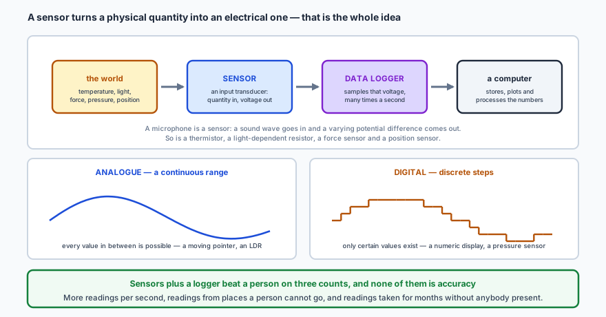
A four-stage chain: the world, carrying quantities such as temperature, light, force, pressure and position; a sensor, described as an input transducer taking a quantity in and giving a voltage out; a data logger, which samples that voltage many times a second; and a computer, which stores, plots and processes the numbers. Below, two graphs contrast an analogue signal, drawn as a smooth continuous curve where every value in between is possible, with a digital signal drawn as a staircase where only certain values exist. A closing note says that sensors with a logger beat a person on three counts, none of them accuracy: more readings per second, readings from places a person cannot go, and readings taken for months without anybody present.
Note what is not on the list of advantages: being more accurate. A logger is not automatically more accurate than a person — it is faster, tireless, and able to be somewhere you are not.
analogue sensora continuous range of values — a moving pointer, an LDR
digital sensordiscrete values only — a numeric display, most modern probes

The three advantages are worth stating precisely, because “it is better” earns nothing:

more detailedmillions of readings a second, and several quantities at once
measured remotelyfrom a place that is inaccessible, or dangerous
measured automaticallyover intervals far too short, or far too long, for a person
The trap: a data logger does not make a measurement more accurate. If a temperature probe is badly calibrated, logging it ten thousand times a second produces ten thousand readings that are all wrong by the same amount — and a beautifully smooth graph of a wrong value. The logger removes human timing error and human tedium. It does nothing at all about systematic error, which is still yours to find.

📊Data you did not take yourself

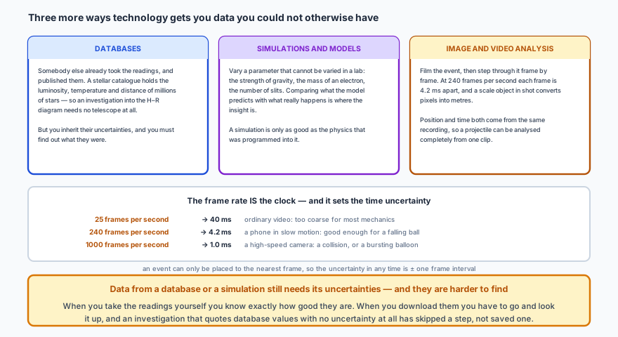
Three cards. Databases: somebody else already took and published the readings, so a stellar catalogue holding the luminosity, temperature and distance of millions of stars lets an investigation into the Hertzsprung-Russell diagram proceed with no telescope, though their uncertainties are inherited and must be looked up. Simulations and models: a parameter that cannot be varied in a laboratory, such as the strength of gravity or the number of slits, can be varied freely, and the insight comes from comparing what the model predicts with what really happens, but a simulation is only as good as the physics programmed into it. Image and video analysis: filming an event and stepping through it frame by frame, with a scale object in shot converting pixels to metres. A table gives frame intervals of 40 milliseconds at 25 frames per second, 4.2 at 240 and 1.0 at 1000.
All three widen what an investigation can be about. All three come with the same catch: you did not control how the data was taken, so you have to go and find out.

Databases hold measurements the scientific community has already made and shared. A stellar catalogue is the obvious example for this course — the whole of E.5 can be investigated from published luminosities, temperatures and parallaxes without owning a telescope.

Simulations and models let you vary what a laboratory will not: the strength of gravity, the mass of a particle, the number of slits. The physics is in the comparison — where the model and reality agree, and more interestingly where they do not.

Image and video analysis extracts both position and time from a single recording. The frame rate is the clock: at 240 frames per second the frames are 4.2 ms apart, and an event can only be placed to the nearest frame, so ± 4.2 ms is the time uncertainty. Include something of known size in the shot and pixels convert into metres.

🔢Spreadsheets and the iterative technique

Some problems have no formula. Drop an object with air resistance and the drag depends on the speed, the speed depends on the acceleration, and the acceleration depends on the drag — each quantity depends on the others and all of them change continuously. There is nothing to substitute into.

The iterative technique gets round this by exploiting a simple fact: over a short enough interval, the acceleration barely changes, and the constant-acceleration equations of A.1 become good enough again. So chop the motion into slices of \( \Delta t \) and step through them.
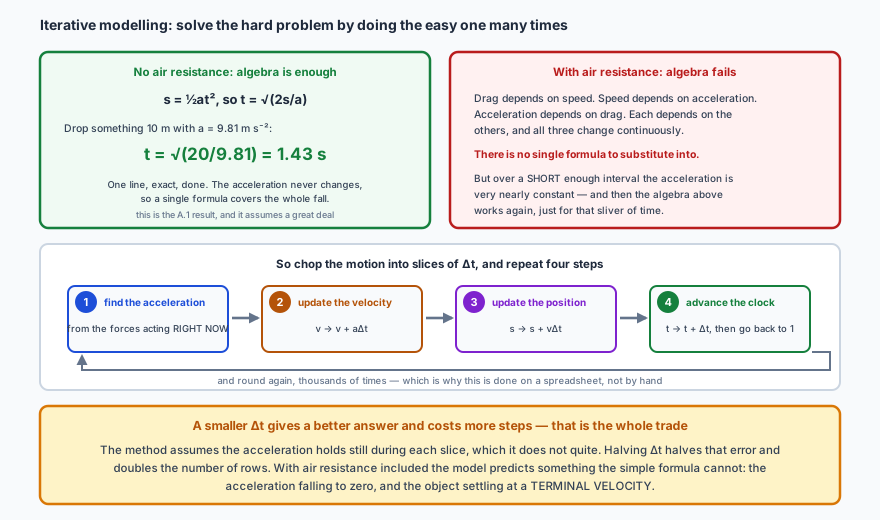
On the left, the case with no air resistance: s equals half a t squared rearranges to t equals the square root of 2s over a, so dropping something 10 metres at 9.81 metres per second squared gives 1.43 seconds in one exact line, because the acceleration never changes. On the right, the case with air resistance: drag depends on speed, speed on acceleration and acceleration on drag, all changing continuously, so there is no single formula to substitute into, but over a short enough interval the acceleration is nearly constant. Below, the iterative loop in four steps: find the acceleration from the forces acting right now, update the velocity to v plus a delta t, update the position to s plus v delta t, advance the clock by delta t and return to step one. A note says a smaller delta t gives a better answer and costs more steps, and that with air resistance the model predicts a terminal velocity that the simple formula cannot.
The loop is four lines of arithmetic repeated thousands of times — trivial for a spreadsheet, unbearable by hand. Each row of the sheet is one time step, and each column is one of the four quantities.

✏️Worked example 1 — the first two rows of an iterative model

An object of mass 0.50 kg is dropped from rest. Air resistance is \( F_d = kv \) with \( k = 0.25 \) N s m−1. Take \( g = 9.81 \) m s−2 and \( \Delta t = 0.10 \) s. Find the velocity after the first two time steps.

Step 1, at \( t = 0 \). The object is at rest, so \( v = 0 \) and there is no drag at all. The only force is the weight:

\[ a = \frac{mg - kv}{m} = \frac{0.50(9.81) - 0}{0.50} = 9.81\ \text{m s}^{-2} \]
\[ v \rightarrow 0 + 9.81(0.10) = 0.981\ \text{m s}^{-1} \]

Step 2, at \( t = 0.10 \) s. Now there is a speed, so there is drag, and the acceleration has already fallen:

\[ a = \frac{0.50(9.81) - 0.25(0.981)}{0.50} = \frac{4.905 - 0.245}{0.50} = 9.32\ \text{m s}^{-2} \]
\[ v \rightarrow 0.981 + 9.32(0.10) = 1.91\ \text{m s}^{-1} \]
Sanity check. The acceleration has dropped from 9.81 to 9.32 in a tenth of a second, which is the physics the constant-acceleration formula cannot represent at all. Continue the loop and \(a\) keeps falling; it reaches zero when \( kv = mg \), that is at \( v = mg/k = 4.905/0.25 = 19.6 \) m s−1 — the terminal velocity. The model predicts it without ever being told it exists, which is the point of the technique.
The trap: a smaller time step is more accurate, not more correct. Every iterative model assumes the acceleration holds still across each slice, and it does not — so every iterative answer carries an error from that assumption. Halving \( \Delta t \) roughly halves that error and exactly doubles the number of rows. It never removes it. If a question asks how to improve such a model, “reduce \( \Delta t \)” is the answer, and “then it would be exact” is not.

✏️Worked example 2 — choosing a frame rate

You want to film a ball falling 1.2 m from rest and measure the time of fall to better than 1%. Would 25 frames per second do? What about 240?

How long is the fall? With no air resistance, \( t = \sqrt{2s/g} = \sqrt{2(1.2)/9.81} = 0.49 \) s.

What uncertainty does each frame rate give? An event can only be placed to the nearest frame, so the uncertainty is one frame interval:

25 fps\( 1/25 = 40 \) ms, and \( 0.040/0.49 = 8.2\% \)
240 fps\( 1/240 = 4.2 \) ms, and \( 0.0042/0.49 = 0.86\% \)

So 25 frames per second misses the target by a factor of eight; 240 just meets it.

Sanity check. The two rates differ by a factor of about ten and the percentages differ by about ten — as they must, since the fall time is the same in both cases. Two practical notes: the uncertainty applies at both ends of the fall, so a careful treatment doubles it; and dropping from a greater height would improve the percentage without needing a better camera at all, which is usually the cheaper fix.

📝Practise

Work through these, then reveal the answer. Each question targets a different objective from the list above.

1. Explain what a sensor does, and why it is also called an input transducer. Give two examples.
A sensor measures a physical quantity and converts it into an electrical signal, usually a potential difference. “Transducer” means a device that converts energy or a signal from one form to another, and “input” because it feeds into the measuring system — so the name describes exactly what it does.
Examples: a microphone converts a sound wave into a varying voltage; a thermistor converts temperature into resistance; a light-dependent resistor does the same for illumination; a force sensor converts an applied force into a voltage. The conversion is what allows a data logger to record the quantity at all.
2. Distinguish an analogue sensor from a digital one, and give an example of each.
An analogue sensor represents the quantity by a continuous range of values, so every value in between is possible — a meter with a moving pointer, or a light-dependent resistor whose resistance varies smoothly with illumination.
A digital sensor represents it using discrete values only, so the output steps between allowed levels — a meter with a numeric display, or a pressure sensor connected to a data logger.
The distinction matters because converting analogue to digital always discards some information: the size of the step is a limit on the resolution, in exactly the way the last digit of a digital display is.
3. State three advantages of using a sensor and data logger rather than taking readings by hand. Is greater accuracy one of them?
Data can be collected more detailed (very many precise readings, and several quantities simultaneously, up to millions per second); remotely (from locations that are difficult, dangerous or simply inaccessible); and automatically (over intervals far too short for a person to react to, or far too long for anybody to sit through).

Greater accuracy is not one of them. A logger removes human reaction time and human tedium, both of which are random effects, so results become more precise and more repeatable. It does nothing about a badly calibrated sensor or a zero error — those are systematic, and logging a wrong value ten thousand times gives ten thousand wrong values.
4. A student investigates the H–R diagram using a published stellar database rather than making observations. State one advantage and one thing they must still do.
Advantage: access to data that could not possibly be collected in a school — luminosities, surface temperatures and parallaxes for many thousands of stars, spanning a range of types no single observing session could cover. New hypotheses can be tested against existing measurements without returning to first principles.
What they must still do: find and quote the uncertainties attached to that data. When you take a reading yourself you know its uncertainty because you chose the instrument; downloaded data carries uncertainties that somebody else determined, and they have to be looked up rather than assumed away. Quoting database values as though they were exact is a real omission, not a saving.
5. Explain why an analytic formula cannot give the motion of a falling object when air resistance is significant.
The drag force depends on the object's speed. The speed depends on the acceleration it has had so far. The acceleration depends on the resultant force, which includes the drag. Each of the three quantities therefore depends on the others, and all of them change continuously throughout the fall.
The constant-acceleration equations assume, as their name says, that \(a\) is constant — which is exactly what is not true here. There is no single expression to substitute into, so the motion must be built up numerically instead.
6. State the four steps of one cycle of an iterative model of motion, in order.
1. Find the acceleration from the resultant force acting at this instant, using \( a = F/m \) with the current velocity substituted into any velocity-dependent force.
2. Update the velocity: \( v \rightarrow v + a\Delta t \).
3. Update the position: \( s \rightarrow s + v\Delta t \).
4. Advance the clock: \( t \rightarrow t + \Delta t \), and return to step 1.
Each cycle is one row of a spreadsheet, and the final values of one row become the starting conditions of the next.
7. An object of mass 0.20 kg falls from rest against a drag force \( F_d = 0.40v \). Using \( \Delta t = 0.05 \) s and \( g = 9.81 \) m s−2, find the velocity after two time steps.
Step 1 (at \(t = 0\), so \(v = 0\) and there is no drag): \[ a = \frac{mg - kv}{m} = \frac{0.20(9.81) - 0}{0.20} = 9.81\ \text{m s}^{-2} \] \[ v \rightarrow 0 + 9.81(0.05) = 0.49\ \text{m s}^{-1} \] Step 2 (now there is drag): \[ a = \frac{0.20(9.81) - 0.40(0.49)}{0.20} = \frac{1.962 - 0.196}{0.20} = 8.83\ \text{m s}^{-2} \] \[ v \rightarrow 0.49 + 8.83(0.05) = 0.93\ \text{m s}^{-1} \] The acceleration has already fallen from 9.81 to 8.83, which is what makes this problem impossible for a single formula.
8. For that same object, find the terminal velocity, and explain how the iterative model reaches it.
Terminal velocity is reached when the resultant force, and therefore the acceleration, falls to zero — that is, when the drag exactly balances the weight: \[ kv = mg \quad \Rightarrow \quad v = \frac{mg}{k} = \frac{0.20 \times 9.81}{0.40} = 4.9\ \text{m s}^{-1} \] The model reaches it without being told it exists. Each cycle, the growing speed makes the drag larger, which makes the resultant force and hence the acceleration smaller, which makes the velocity grow more slowly. The velocity therefore approaches 4.9 m s−1 asymptotically and the acceleration approaches zero. That emergent behaviour is the main reason for modelling this way.
9. What happens to an iterative model's accuracy and its cost when \( \Delta t \) is halved? Can \( \Delta t \) be made small enough to give an exact answer?
Halving \( \Delta t \) roughly halves the error and exactly doubles the number of steps — twice as many rows for a computer to work through. That is the whole trade-off.
It cannot be made exact. The method's error comes from assuming the acceleration is constant across each slice, and that assumption is wrong for every non-zero \( \Delta t \), however small. The error can be made as small as you have patience and computing time for, but it never reaches zero. Saying that a small enough step would make the model exact is the misconception to avoid.
10. A collision lasts about 15 ms. A student films it at 120 frames per second. Explain whether this is adequate, and what they should do instead.
At 120 frames per second the interval between frames is \( 1/120 = 8.3 \) ms. A 15 ms collision therefore spans fewer than two frame intervals — the student would capture perhaps one frame during the collision itself, which is not enough to see anything happen, let alone measure it.
They need a much higher frame rate: at 600 frames per second the interval is 1.7 ms, giving roughly nine frames across the collision, which is enough to track the deformation and find the contact time. Alternatively, use a force sensor connected to a data logger, which can sample far faster than any affordable camera and gives the force directly rather than requiring it to be inferred from positions.

🔗Go deeper — other people’s work

These are external resources, not mine. If one stops working, tell me and everything above it on this page still stands.

  • Tracker — free video-analysis software, and the standard tool for this kind of work
  • PhET — simulations across the whole DP syllabus, useful for the modelling half of this topic