Market failure: market power
🎯What you need to be able to do
- HL Describe perfect competition, monopoly, oligopoly and monopolistic competition by number of firms, barriers to entry and type of product.
- HL Explain profit maximization (TR − TC, MR = MC) and abnormal profit, normal profit and losses; calculate profit, MC, MR, AC and AR from data.
- HL Draw the perfectly competitive firm as a price taker, with abnormal profit, normal profit and losses in the short run, and long-run equilibrium with allocative efficiency (P = MC).
- HL Draw a monopolist making abnormal profit, normal profit and losses; compare monopoly with perfect competition, including the welfare loss; draw a natural monopoly.
- HL Explain oligopoly: collusion and cartels, interdependence, price wars, a simple game-theory payoff matrix, price and non-price competition, concentration ratios.
- HL Draw monopolistic competition in the short and long run.
- HL Evaluate the advantages and risks of large firms with market power, and government responses: legislation and regulation, government ownership and fines.
📚The economics
Four market structures
many small firms; homogeneous (identical) products; free entry and exit; perfect information. Each firm is a price taker. Closest real cases: some agricultural and commodity markets, foreign exchange.
many firms; differentiated products; free entry and exit. Some price-setting power. Cafés, hair salons, warung, clothing boutiques.
a few large firms dominate; high barriers to entry; interdependence: each firm must consider rivals’ reactions. Mobile networks, cement, airlines, soft drinks.
a single (or dominant) firm; high barriers to entry; no close substitutes. Price maker. State electricity distribution, patented medicines, local water supply.
Barriers to entry protect market power: economies of scale, legal barriers (patents, licences), control of essential resources, high set-up costs, brand loyalty, network effects, and aggressive tactics by incumbents.
Revenue, cost and profit
Average revenue AR = TR ÷ Q = P (so AR is the demand curve)
Marginal revenue MR = ΔTR ÷ ΔQ
Average cost AC = TC ÷ Q
Marginal cost MC = ΔTC ÷ ΔQ
Economic costs include opportunity costs, including the return the owners could earn elsewhere. So:
TR = TC: the minimum profit needed to keep the firm in the industry. Zero economic profit.
TR > TC: profit above normal. Attracts entry if barriers allow.
TR < TC. In the long run, loss-makers leave.
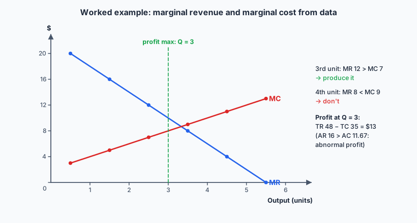
Profit maximization: MR = MC. If the next unit adds more to revenue than to cost (MR > MC), produce it; if it adds more to cost (MR < MC), don’t. Profit is greatest where MR = MC (with MC rising through MR).
Perfect competition: no market power
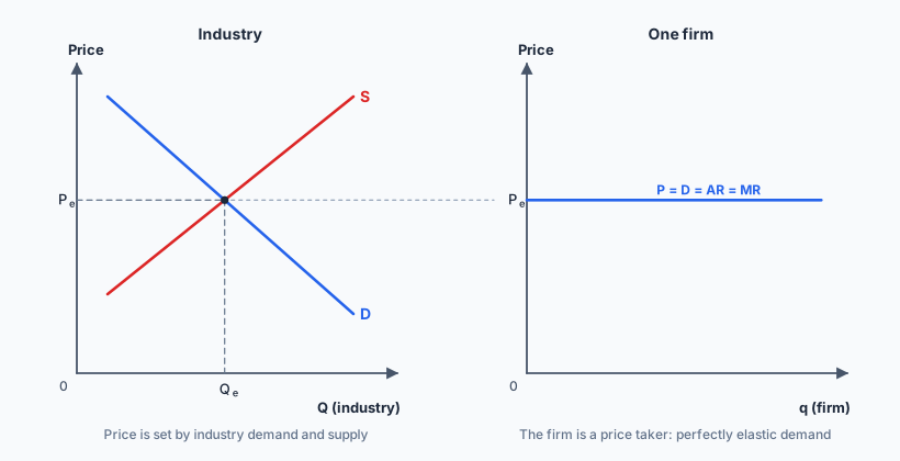
Because there are many sellers of an identical product, each firm’s output is too small to affect the price. It must accept the market price set by industry demand and supply. If it charged more it would sell nothing; it can sell as much as it likes at the market price. So the firm’s demand curve is perfectly elastic, and P = D = AR = MR.
Short run. The firm produces where MR (= P) = MC. Whether it makes a profit depends on where the price lies relative to its AC:
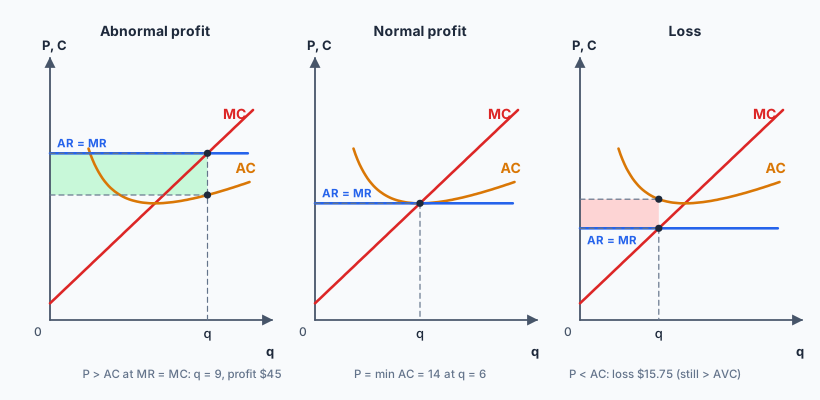
A loss-making firm continues in the short run as long as the price covers its average variable cost (it contributes something to fixed costs, which must be paid anyway). If price falls below AVC, it shuts down immediately.
Long run. Abnormal profits attract new firms (no barriers), so industry supply shifts right and the price falls until only normal profit remains. Losses make firms leave, supply shifts left and the price rises. Long-run equilibrium: P = MR = MC = minimum AC, normal profit only.
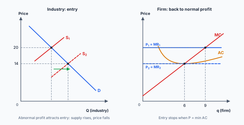
Efficiency: in long-run equilibrium, P = MC means price (the marginal benefit to consumers) equals marginal cost: allocative efficiency, with social surplus maximized (MB = MC). Firms also produce at minimum AC: productive efficiency. This is the benchmark for judging the other structures.
Monopoly
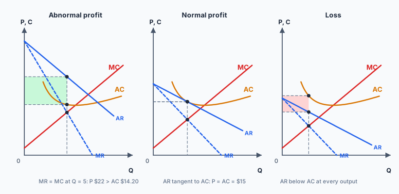
A monopolist faces the whole downward-sloping market demand curve. To sell one more unit it must lower the price on all units, so MR lies below AR (for a straight-line demand curve, MR has twice the slope). It maximizes profit at MR = MC, then charges the highest price consumers will pay for that output, read off the AR curve. Because barriers block entry, abnormal profit can persist in the long run.
Monopoly compared with perfect competition. Suppose a competitive industry is taken over by a single firm with the same costs (constant MC = AC).
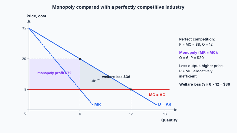
- Higher price, lower output: $20 and 6 units, against $8 and 12.
- Allocative inefficiency: P ($20) > MC ($8). Consumers value units 7 to 12 above their cost, yet they are not produced: a welfare loss of ½ × 6 × 12 = $36. This is market failure.
- Redistribution: part of consumer surplus ($72 here) becomes monopoly profit.
- Possible X-inefficiency (costs higher than necessary without competitive pressure) and less choice.
Natural monopoly. Where economies of scale are so large that average costs keep falling over the whole range of market demand, one firm can supply the market more cheaply than two or more. Electricity grids, water pipes, rail track and gas networks are examples: duplicating them would waste resources.
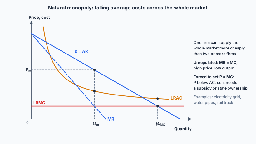
This creates a dilemma. Left alone, a natural monopoly charges a high price. Forced to price at MC (allocative efficiency), it makes a loss because P < AC. Governments therefore often own natural monopolies (Indonesia’s PLN electricity and PAM water companies) or regulate their prices (for example average-cost pricing, P = AC).
Oligopoly
A few firms dominate, so each firm’s best decision depends on what its rivals do: interdependence.
- Collusive oligopoly: firms cooperate to limit competition, usually to fix prices or share markets. A formal agreement is a cartel (OPEC coordinating oil output is the best-known international example). Colluding firms act together like a monopoly: they set joint MR = MC and share the abnormal profit, so the monopoly diagram above applies. Most countries ban collusion; Indonesia’s competition authority, KPPU, has brought cartel cases in several industries, including cooking oil.
- Tacit collusion: no formal agreement, but firms follow a price leader or avoid price cuts.
- Non-collusive oligopoly: firms compete, but are wary of price wars: if one cuts price, rivals match it and all lose profit. So prices tend to be stable, and firms compete through non-price competition: advertising, branding, loyalty schemes, product features, after-sales service.
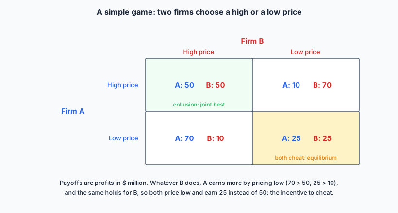
Game theory models interdependent decisions. In the payoff matrix below, both firms would be best off colluding on a high price (50 each), but each has an incentive to cheat: whatever the rival does, pricing low earns more. So both price low and earn 25: the prisoner’s dilemma. This explains why cartels are unstable, and why firms still try to collude.
Concentration ratios measure how dominated a market is. The n-firm concentration ratio (CRn) is the combined market share of the n largest firms. A four-firm ratio (CR4) above about 50% suggests oligopoly; close to 100% for one firm indicates monopoly. Limitations: they ignore the relative sizes within the top n, foreign competition, and how contestable the market is.
Monopolistic competition
Many firms sell differentiated products, so each has a downward-sloping demand curve, but because there are many close substitutes it is much more elastic than a monopolist’s.
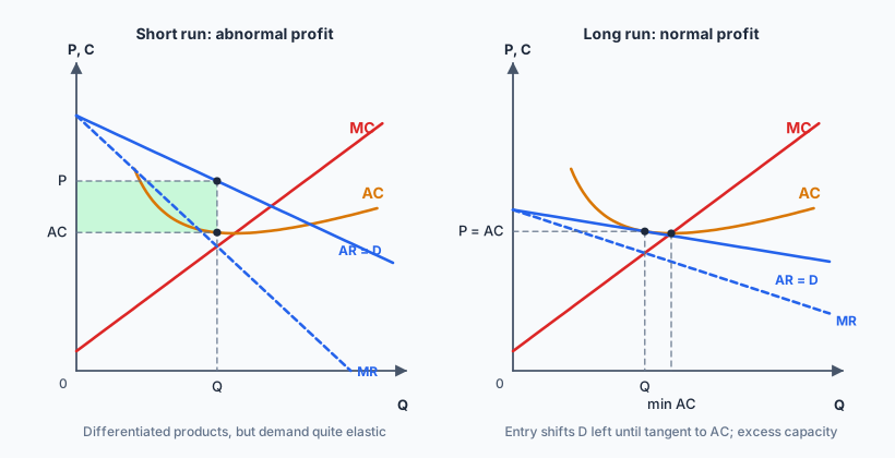
- Short run: abnormal profit (or losses) are possible, exactly as in the monopoly diagram.
- Long run: abnormal profit attracts new firms with similar products (free entry). Each firm’s demand curve shifts left (and becomes more elastic) until it is tangent to AC: normal profit. Losses cause exit, shifting demand right.
- Efficiency: P > MC, so it is allocatively inefficient, but less so than monopoly because demand is more elastic. Firms produce below minimum AC (excess capacity), so not productively efficient.
- Benefit: more product variety and choice, which consumers value.
Large firms with market power: advantages and risks
Economies of scale lower average costs, which can mean lower prices than many small firms could charge (natural monopolies especially). Abnormal profits finance research and development, hence innovation: new medicines, technology platforms. Stable firms can invest long-term and compete internationally.
Output restricted and prices higher than under competition; less consumer choice; allocative inefficiency and welfare loss; X-inefficiency; power over suppliers and workers; political lobbying; abuse such as predatory pricing or tying products together to exclude rivals.
Government responses to abuse of market power
- Legislation and regulation (competition policy): laws banning cartels and abuse of dominance; blocking mergers that would reduce competition; price caps on regulated monopolies (utilities). Indonesia’s competition law (1999) is enforced by KPPU.
- Fines: penalties for anti-competitive behaviour. The European Commission fined Google €2.42 billion (2017) over its shopping comparison service and €4.34 billion (2018) over Android.
- Government ownership: the state runs the natural monopoly itself, pricing for social goals (PLN, PAM water).
- Other options: breaking up dominant firms; promoting entry (deregulation, trade liberalization, 3.7).
Evaluation: regulators may lack information about costs, may be captured by the industry, and cases take years; fines may be small relative to profits; breaking up firms can sacrifice economies of scale. Dynamic markets (technology) also change faster than regulation.
✏️Worked example HL
0, 1, 2, 3, 4, 5, 6
22, 20, 18, 16, 14, 12, 10
20, 23, 28, 35, 44, 55, 68
(b) Identify the profit-maximizing output and calculate the profit.
(c) Is this abnormal profit? Use AR and AC.
(a) TR = P × Q: 0, 20, 36, 48, 56, 60, 60. MR (change in TR): 20, 16, 12, 8, 4, 0. MC (change in TC): 3, 5, 7, 9, 11, 13.
(b) Produce each unit while MR ≥ MC: unit 3 has MR 12 > MC 7, unit 4 has MR 8 < MC 9. So Q = 3. Profit = TR − TC = 48 − 35 = $13. (Check: profit at Q = 2 is 36 − 28 = 8 and at Q = 4 is 56 − 44 = 12, both lower.)
(c) AR = $16; AC = 35 ÷ 3 = $11.67. AR > AC, so it is abnormal profit: (16 − 11.67) × 3 = $13.
📝Practise
All HL. Tagged questions are modelled on a real IB question from that session, with our own wording and context.
1. [2 marks, Paper 2 style] The four largest firms in a market have sales of $40 m, $25 m, $15 m and $10 m. Total market sales are $120 m. Calculate the four-firm concentration ratio.
2. [10 marks, Paper 1 (a) — modelled on May 2024 HL Paper 1 Q1(a)] Using diagrams, explain what happens to a price-taking firm’s profit, and to the number of firms in the industry, after a permanent rise in market demand.
Define perfect competition (many firms, homogeneous product, free entry and exit, perfect information) and abnormal profit (AR > AC). Short run: an increase in demand raises the market price; the price-taking firm produces where P = MR = MC, with P > AC: abnormal profit (firm and industry diagrams).
Long run: perfect information means outsiders see the profit, and with no barriers they enter. Industry supply shifts right and the price falls until P = min AC, so only normal profit remains (two-panel long-run diagram). Explain each step of the adjustment in words linked to the diagram.
3. [10 marks, Paper 1 (a) — modelled on November 2024 HL Paper 1 Q1(a)] Explain why barriers to entry let a monopolist keep earning abnormal profit that a café owner in a busy tourist town cannot.
4. [15 marks, Paper 1 (b) — modelled on May 2023 HL Paper 1 Q1(b)] Using real-world examples, evaluate whether consumers are better served by a market of many small firms selling differentiated products or by one dominated by a few large firms.
For monopolistic competition: more elastic demand, so less allocative inefficiency; only normal profit in the long run (prices closer to cost); lots of variety and choice; free entry keeps firms responsive; no collusion risk (too many firms).
For oligopoly: economies of scale can mean lower costs and prices; abnormal profits fund R&D (pharmaceuticals, smartphones); non-price competition drives quality and innovation; competition between a few large firms can still be fierce (airlines, telecoms price wars).
Against oligopoly: collusion and cartels, high prices, barriers. Against monopolistic competition: excess capacity, waste on advertising, small firms cannot afford R&D.
Judgment: depends on the industry (cafes suit monopolistic competition; steel, telecoms or aircraft making need scale), on whether oligopolists collude, and on the strength of competition policy.
5. [15 marks, Paper 1 (b) — modelled on November 2023 HL Paper 1 Q1(b)] Using real-world examples, examine the options open to a competition authority when four firms control most of a country’s cement market.
Explain concentration ratios and why high concentration may mean market power (oligopoly or monopoly), with a diagram of monopoly/collusive oligopoly and welfare loss.
Responses: investigate and ban collusion (fines, as in EU competition cases); block mergers; regulate prices (price caps on utilities); government ownership of natural monopolies; encourage entry (deregulation, lower trade barriers, support for small firms).
Evaluation: high concentration is not proof of abuse (economies of scale, contestable markets, international competition); regulators’ information problems; risk of government failure; the cost of breaking up efficient firms. Conclude with a context-dependent judgment.
6. Explain, with a diagram, why a natural monopoly is often owned or regulated by the government.
🔗Go deeper — other people’s work
These are external resources, not mine. If one stops working, tell me and everything above it on this page still stands.
- Khan Academy — Forms of competition unit: perfect competition, monopoly, oligopoly and game theory.
- European Commission competition cases database — decisions and fines against Google and others.
- KPPU (Indonesia’s Business Competition Supervisory Commission) — published decisions on cartels and mergers.