Aggregate demand and aggregate supply
🎯What you need to be able to do
- Draw and explain the AD curve; explain its components C + I + G + (X − M) and their determinants; show shifts of AD.
- Draw and explain the SRAS curve, its determinants (costs of factors of production, indirect taxes) and shifts.
- Explain the monetarist/new classical LRAS and the Keynesian AS curve, and inflationary and deflationary (recessionary) gaps.
- Explain the causes of shifts in LRAS / Keynesian AS: quantity and quality of factors, technology, efficiency and institutions.
- Draw short-run and long-run equilibrium in both models: automatic adjustment and the natural rate of unemployment in the monetarist model; persistent deflationary gaps in the Keynesian model.
- Evaluate the assumptions and implications of the two models.
📚The economics
Aggregate demand
Aggregate demand (AD) is the total planned spending on an economy’s final goods and services at each price level, in a given period.
The AD curve slopes downwards: at a lower average price level, the real value of households’ money and savings is higher (wealth effect), interest rates tend to be lower (interest rate effect, encouraging borrowing), and domestic goods are cheaper relative to foreign ones (trade effect). A change in the price level is a movement along AD; a change in any component shifts it.
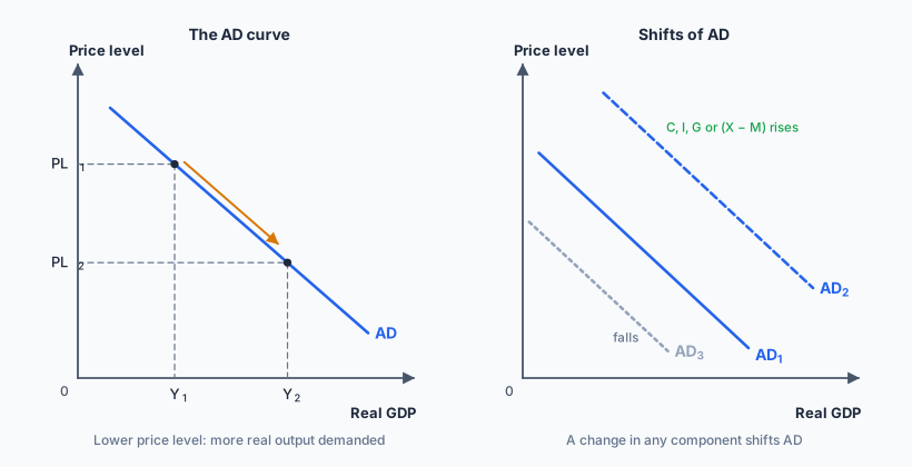
Determinants of the components of AD
- Consumption (C), household spending, the largest component (over half of Indonesia’s GDP): consumer confidence; interest rates (the cost of borrowing and reward for saving); wealth (house and share prices); income taxes; household indebtedness; expectations of future prices.
- Investment (I), firms’ spending on capital goods: interest rates; business confidence; technology (new processes to invest in); business taxes; corporate indebtedness.
- Government spending (G): political and economic priorities (infrastructure programmes, stimulus during recessions, election promises such as Indonesia’s free school meals programme from 2025).
- Net exports (X − M): incomes of trading partners (China’s growth drives demand for Indonesian coal and nickel); exchange rates (a weaker rupiah makes exports cheaper and imports dearer); trade policies (tariffs, trade agreements).
Short-run aggregate supply
SRAS shows the total output firms plan to produce at each price level in the short run, when the prices of factors of production, especially wages, are fixed (by contracts, for example). If the price level rises while costs stay fixed, production becomes more profitable, so output rises: SRAS slopes upwards.
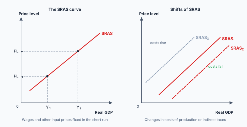
Shifts of SRAS come from changes in costs of factors of production (wages, rents, oil and other raw-material prices, imported inputs when the exchange rate falls) and indirect taxes (a rise in VAT shifts SRAS left). A subsidy to producers shifts it right. Supply shocks such as the 2022 energy price spike shift SRAS sharply left.
Two views of aggregate supply in the long run
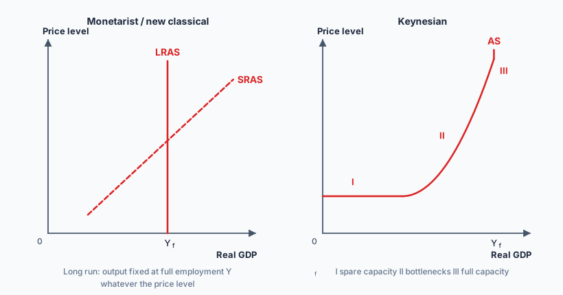
In the long run, wages and prices are fully flexible. Output is determined by the economy’s resources and technology, not by the price level, so the LRAS is vertical at the full employment level of output (potential output, Yf). Changes in AD affect only the price level in the long run.
Wages and prices are sticky downwards (contracts, unions, minimum wages, reluctance to cut pay). The AS curve has three sections: I horizontal, with lots of spare capacity, so output can rise with no inflation; II rising, as bottlenecks and shortages of skilled labour appear; III vertical at full capacity.
Inflationary and deflationary gaps
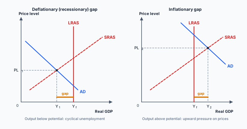
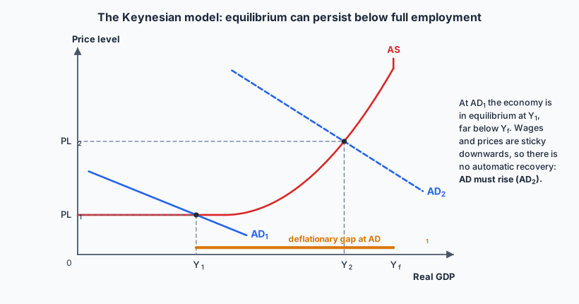
- Deflationary (recessionary) gap: equilibrium real GDP is below potential output. There is unemployment above the natural rate (cyclical unemployment) and spare capacity.
- Inflationary gap: equilibrium real GDP is above potential output: firms use overtime, overstretch capacity and compete for scarce labour, so costs and prices rise.
Shifts of LRAS and the Keynesian AS
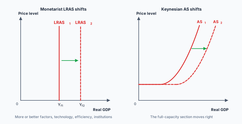
- Quantity of factors of production: more labour (population growth, migration, higher participation), more capital (investment), new resources.
- Quality of factors: education, training and health (human capital); better infrastructure.
- Improvements in technology: automation, digital platforms, better seeds.
- Increases in efficiency: more competition, better management, reallocation of resources to more productive uses.
- Changes in institutions: secure property rights, less corruption and red tape, stable legal and banking systems, labour market reforms. (Supply-side policies, 3.7, target all of these.)
Macroeconomic equilibrium
Short-run equilibrium is where AD = SRAS. Long-run behaviour is where the schools differ.
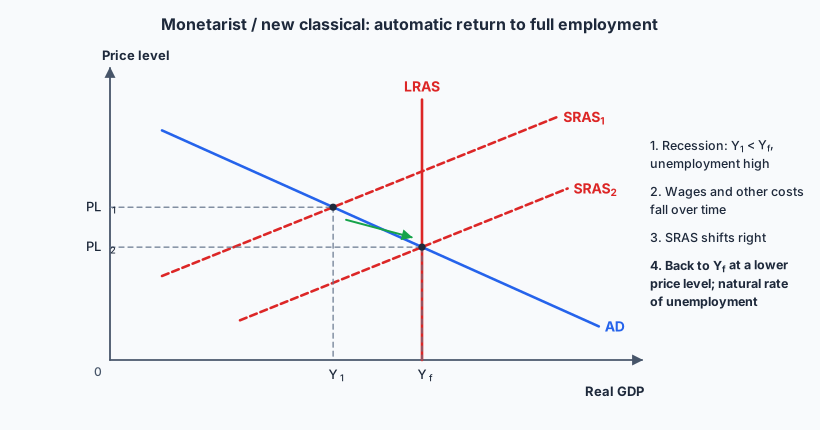
Monetarist / new classical model. Long-run equilibrium is where AD = SRAS = LRAS, at full employment output. The economy adjusts automatically: in a recession, unemployment puts downward pressure on wages and other costs, SRAS shifts right, and output returns to Yf at a lower price level. In a boom, rising wages shift SRAS left until output is back at Yf with higher prices. At full employment, unemployment is not zero but equal to the natural rate of unemployment (structural + frictional + seasonal, 3.3).
Keynesian model. Because wages and prices do not fall easily, a recession can persist: the economy can be in equilibrium in section I of the AS curve, with a deflationary gap and high unemployment, for a long time. Pessimism can make it worse: falling incomes cut consumption, which cuts output further. Recovery needs AD to rise, so the government should intervene (demand management, 3.6).
Assumptions and implications of the two models
Assumes flexible wages and prices, rational agents and self-correcting markets. Implication: demand-side policy cannot raise output permanently, only the price level; governments should keep inflation low and stable and use supply-side policies to raise potential output. Intervention risks inflation and government failure.
Assumes sticky wages and prices, that expectations and confidence matter, and that markets can fail to clear for long periods. Implication: governments should actively manage AD, especially in recessions, through fiscal policy. “In the long run we are all dead”: waiting for self-correction is too costly.
Evidence supports parts of both: long recessions (the 1930s, Japan in the 1990s, the 2008–09 crisis) suggest slow self-correction, while 1970s stagflation and high inflation after large stimulus suggest limits to demand management.
✏️Worked example
(a) Lower borrowing costs raise C and I: AD shifts right. Price level ↑, real GDP ↑ (by how much depends on how close the economy is to full capacity).
(b) Higher costs for firms: SRAS shifts left. Price level ↑, real GDP ↓: cost-push inflation, possibly stagflation.
(c) Lower foreign incomes reduce demand for exports, so X falls: AD shifts left. Price level ↓ (or rises more slowly), real GDP ↓.
(d) Better-quality labour raises productive capacity: LRAS (Keynesian AS) shifts right. Potential output ↑, downward pressure on the price level.
📝Practise
Tagged questions are modelled on a real IB question from that session, with our own wording and context.
1. [2 marks, Paper 2 style] Define the term aggregate demand.
2. [10 marks, Paper 1 (a) — modelled on November 2023 SL Paper 1 Q2(a)] Explain, with an AD/AS diagram, how a wave of consumer optimism and a rise in the central bank’s policy rate would each affect real output in the short run.
Consumer confidence rises: households are more optimistic about jobs and income, so they spend more and save less: C rises, AD shifts right, and in the short run the price level and real GDP both rise (AD/AS diagram with SRAS).
Interest rates rise: borrowing becomes dearer and saving more rewarding, so credit-financed consumption and investment fall; mortgage payments rise, cutting disposable income: AD shifts left, price level and real GDP fall. If both happen together, the net effect depends on their relative strength. Two diagrams, clearly labelled.
3. [10 marks, Paper 1 (a) — modelled on November 2023 SL Paper 1 Q2(a)] Explain how new automation technology and a larger pool of trained technicians would affect an economy’s full employment output.
4. [10 marks, Paper 1 (a) — modelled on November 2024 HL Paper 1 Q2(a)] Using an AD/AS diagram, explain how, according to monetarist/new classical economists, an economy recovers from a recession without government action.
5. Explain why the Keynesian AS curve is horizontal at low levels of real GDP.
6. [4 marks, Paper 2 style] Using an AD/AS diagram, explain the likely effect on real GDP of a sharp rise in global energy prices for an energy-importing country.
🔗Go deeper — other people’s work
These are external resources, not mine. If one stops working, tell me and everything above it on this page still stands.
- Khan Academy — Aggregate demand and aggregate supply unit.
- Bank Indonesia — Monetary Policy Report, which discusses the drivers of Indonesian demand and inflation each quarter.
- Marginal Revolution University — Principles of Macroeconomics videos on the AD/AS model.