Supply
🎯What you need to be able to do
- Define supply and explain the law of supply, drawing an upward-sloping supply curve.
- Explain the relationship between an individual producer’s supply and market supply.
- Explain the non-price determinants of supply: costs of factors of production, prices of related goods (joint and competitive supply), indirect taxes and subsidies, future price expectations, technology and the number of firms.
- Distinguish between movements along and shifts of the supply curve, with diagrams.
- HL Explain the assumptions underlying the law of supply: the law of diminishing marginal returns and increasing marginal costs.
📚The economics
Supply and the law of supply
Supply is the quantity of a good or service that producers are willing and able to supply at each possible price, in a given time period, ceteris paribus.
The law of supply states that there is a positive (direct) relationship between price and quantity supplied, ceteris paribus: as the price rises, quantity supplied rises. Two reasons:
- A higher price makes production more profitable, so existing firms produce more and switch resources from less profitable products.
- Producing more usually raises the cost of each extra unit, so firms need a higher price to cover it (the HL explanation below).
Why the supply curve slopes upwards HL
In the short run, at least one factor of production is fixed: a factory’s size, a farm’s land. Firms raise output by adding variable factors such as labour.
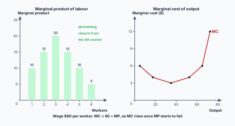
- The law of diminishing marginal returns: as more units of a variable factor are added to a fixed factor, the marginal product (extra output from one more unit) eventually falls. The fifth worker on a small farm has less land and fewer tools to work with than the first.
- Increasing marginal costs: if each extra worker costs the same wage but adds less output, the cost of each extra unit of output rises. Marginal cost (MC) = wage ÷ marginal product. Firms supply more only if the price covers this rising MC, so the supply curve is the firm’s marginal cost curve (above its minimum average variable cost).
Individual and market supply
Market supply is the sum of the quantities supplied by all firms at each price: a horizontal summation of the individual supply curves, exactly as for demand. More firms in the market means more market supply.
Non-price determinants of supply
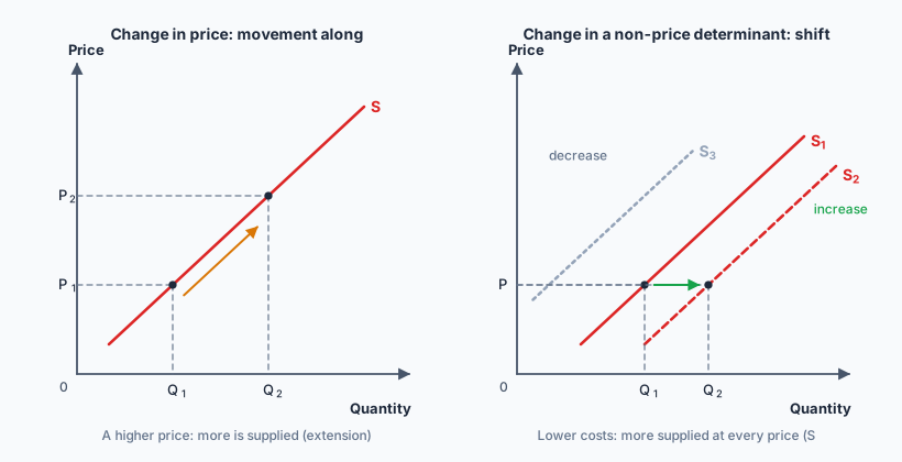
These shift the supply curve. An increase in supply is a shift to the right (more supplied at every price, or the same amount at a lower price); a decrease is a shift to the left.
- Costs of factors of production. Higher wages, rents, fuel or raw material prices raise costs and decrease supply. When Indonesia raised subsidized fuel prices in September 2022, transport and fishing costs rose and supply of many goods shifted left.
- Prices of related goods. Competitive supply: goods that use the same resources (a farmer can grow maize or soybeans on the same land). If the price of maize rises, farmers switch land to maize, so supply of soybeans decreases. Joint supply: goods produced together (beef and leather, crude oil refined into petrol and diesel). If the price of beef rises, more cattle are slaughtered, so supply of leather increases.
- Indirect taxes and subsidies. A tax per unit is an extra cost, so supply decreases (shifts up/left by the tax). A subsidy per unit lowers costs, so supply increases (2.7).
- Future price expectations. If producers expect prices to rise, they may hold back stock now to sell later, decreasing current supply. (For farmers who can plant more, expected higher prices may instead increase supply later.)
- Changes in technology. Better technology raises productivity and lowers costs: supply increases. Drip irrigation, better seed varieties and automation are examples.
- Number of firms. New entrants increase market supply; firms leaving decrease it.
- Also: natural events such as droughts, floods and volcanic eruptions shift agricultural supply sharply, which is why food prices are volatile.
Movements along and shifts of the supply curve
✏️Worked example HL
1, 2, 3, 4, 5, 6
10, 25, 45, 60, 70, 75
(b) Calculate the marginal cost of a loaf for each worker’s output.
(c) Identify where diminishing marginal returns set in, and explain the link to the supply curve.
(a) Marginal product = change in total output from one more worker: 10, 15, 20, 15, 10, 5.
(b) MC per loaf = wage ÷ marginal product: 60 ÷ 10 = $6, 60 ÷ 15 = $4, 60 ÷ 20 = $3, then $4, $6, and 60 ÷ 5 = $12.
(c) Marginal product is highest for the 3rd worker and falls from the 4th worker onwards: diminishing marginal returns set in because more workers share one oven. From then on, each extra loaf costs more ($4, $6, $12). The bakery will only produce the extra loaves if the price covers this rising marginal cost, so it supplies more only at higher prices: an upward-sloping supply curve.
📝Practise
Work through these on paper, then reveal the answer. Tagged questions are modelled on a real IB question from that session, with our own wording and context.
1. [2 marks, Paper 2 style] Define the term supply.
2. [4 marks, Paper 2 style] Using a demand and supply diagram, explain the effect on the market for chilli peppers of heavy rains that destroy part of the harvest.
3. [10 marks, Paper 1 (a) — modelled on November 2024 SL Paper 1 Q1(a)] Distinguish, with diagrams, between the effect of a drought on the market for coffee beans and the effect of a higher coffee price on growers’ output.
A fall in supply (for example after a drought in coffee-growing regions) is a change in a non-price determinant: the supply curve shifts left. At the original price, quantity demanded now exceeds quantity supplied (a shortage); buyers compete for the limited beans and the price rises until a new, higher equilibrium is reached with a smaller quantity.
A rise in price by itself causes a movement along the supply curve: quantity supplied extends. Higher prices raise profitability, give an incentive to devote more land and labour to coffee, and cover the rising marginal cost of extra output (diminishing marginal returns at HL).
Two labelled diagrams, the distinction between “supply” and “quantity supplied”, and a real example lift this into the top band.
4. Explain the difference between joint supply and competitive supply, with an example of each.
5. HL A firm’s marginal product of labour falls from 40 to 25 units while the wage stays at $50. Calculate the change in marginal cost and explain its significance.
6. For the market for rice in Indonesia, state the direction of the supply shift in each case: (a) a new high-yield rice variety; (b) higher fertilizer prices; (c) the government pays farmers a subsidy per tonne; (d) many farmers convert paddy fields to housing.
🔗Go deeper — other people’s work
These are external resources, not mine. If one stops working, tell me and everything above it on this page still stands.
- Khan Academy — Law of supply and Changes in supply versus quantity supplied.
- Marginal Revolution University — The supply curve and What shifts supply?
- FAO Food Price Index — monthly data showing how weather and costs shift supply of food commodities.