Macroeconomic objectives
🎯What you need to be able to do
- Explain short-term growth (PPC, AD) and long-term growth (PPC shift, LRAS); calculate the growth rate; evaluate the consequences of growth for living standards, the environment and income distribution.
- Calculate the unemployment rate; explain difficulties of measurement; explain cyclical, structural, seasonal and frictional unemployment, the natural rate, and the costs of unemployment.
- Calculate inflation from CPI data; explain the limitations of the CPI; explain demand-pull and cost-push inflation, deflation and disinflation, and the costs of each.
- Evaluate the relative costs of unemployment and inflation, and conflicts between objectives: growth and inflation, growth and sustainability, growth and equity.
- HL Calculate a weighted price index; explain sustainable government debt; explain the short-run and long-run Phillips curves.
📚The economics
1. Economic growth
Economic growth is an increase in real GDP (or real GDP per capita) over time.
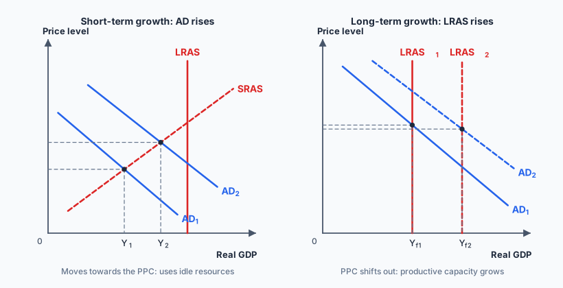
Output rises by using idle resources: a movement from inside the PPC towards it (1.1). In AD/AS, an increase in AD when there is a deflationary gap.
Productive capacity rises: an outward shift of the PPC, and a rightward shift of LRAS, from more or better factors, technology and institutions.
Consequences of growth:
- Living standards: higher incomes, more goods and services, more tax revenue for health and education, lower absolute poverty. Indonesia’s long run of about 5% annual growth has cut extreme poverty sharply since 2000. But more output does not guarantee better lives: working hours, stress, congestion and pollution may rise.
- Environment: growth based on fossil fuels, deforestation and resource extraction causes pollution, climate change and depletion (4.7). Growth can also fund cleaner technology and, at higher incomes, people demand a cleaner environment.
- Income distribution: growth may benefit owners of capital and skilled workers most, widening inequality; or, if broad-based (labour-intensive manufacturing, rural development), it can reduce it.
2. Low unemployment
A person is unemployed if they are of working age, without work, available for work and actively looking for it. The labour force is the employed plus the unemployed.
Difficulties of measuring unemployment:
- Hidden unemployment: discouraged workers who have given up looking are not counted.
- Underemployment: part-time workers who want full-time work, and graduates in jobs that do not use their skills, count as employed.
- The informal economy: many people in developing countries (well over half of Indonesia’s workers) work informally, so “employed” hides very low and insecure incomes.
- An average hides disparities between regions, ages (youth unemployment is usually much higher), genders and ethnic groups.
Types (causes) of unemployment:
- Cyclical (demand-deficient): caused by a fall in AD in a recession. Firms cut output and jobs. Shown by a deflationary gap (3.2).
- Structural: a mismatch between the skills or locations of workers and the jobs available, caused by changes in demand patterns, technology (automation) or the decline of industries. Long-lasting. Shown by a fall in demand for a particular type of labour. Also caused by labour market rigidities, such as a minimum wage above equilibrium, generous benefits or strong unions.
- Frictional: short-term unemployment while people move between jobs or search for their first job. Inevitable in a dynamic economy.
- Seasonal: demand for labour varies with the seasons: agriculture between harvests, tourism in the low season (Bali’s hotels hire fewer workers outside the peak months).
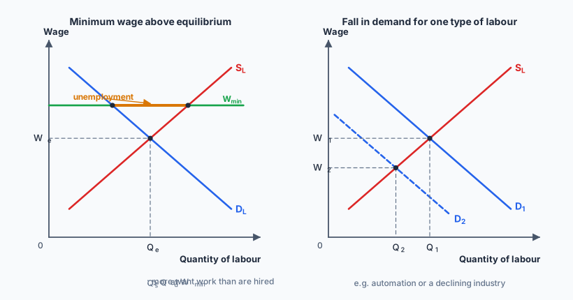
The natural rate of unemployment is the sum of structural, frictional and seasonal unemployment: the unemployment that remains when the economy is at full employment (Yf). Full employment therefore does not mean zero unemployment. Demand-side policy can remove cyclical unemployment; the natural rate needs supply-side policy.
Costs of unemployment:
loss of income; loss of skills (the longer unemployed, the harder to find work); stress, health problems, family breakdown.
crime, social unrest, homelessness, inequality and poverty; unemployment concentrated in regions or groups.
lost output (a point inside the PPC); lower tax revenue and higher spending on benefits; lower demand for other firms’ products; loss of human capital.
3. Low and stable inflation
Inflation is a sustained rise in the average price level. Deflation is a sustained fall in the price level. Disinflation is a fall in the rate of inflation (prices still rising, but more slowly). Many central banks target around 2%; Bank Indonesia’s target is 2.5% ± 1% (for 2024 onwards).
Measuring inflation: the consumer price index (CPI). Statisticians survey household spending to find a representative basket of goods and services and the weights (share of spending) of each. Prices are collected regularly, and a weighted price index is calculated with a base year = 100. The inflation rate is the percentage change in the CPI.
Limitations of the CPI: the basket represents an average household, not the poor, the elderly or rural families whose spending patterns differ; weights go out of date; quality improvements are hard to allow for, so the CPI may overstate inflation; new products enter the basket late; consumers substitute towards goods that have become relatively cheaper; different regions face different price changes; and informal-market prices are hard to collect.
Causes of inflation:
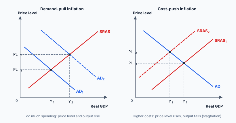
caused by an increase in AD, especially near full capacity: rising consumer spending, investment booms, government spending, export demand, rapid credit growth. “Too much money chasing too few goods.”
caused by a decrease in SRAS from rising costs: higher oil and food prices, wage rises not matched by productivity, a depreciating currency raising import prices, higher indirect taxes. Can cause stagflation: inflation with falling output.
Costs of high inflation:
- Uncertainty: firms cannot plan, so investment falls.
- Redistributive effects: people on fixed incomes (pensioners, many workers) lose purchasing power; borrowers gain and lenders lose as the real value of debt falls.
- Effects on saving: if inflation exceeds the interest rate, the real value of savings falls, discouraging saving.
- Damage to export competitiveness: exports become relatively expensive, imports relatively cheap; the current account worsens.
- Impact on economic growth: less investment and saving reduce long-term growth.
- Inefficient resource allocation: price signals are distorted; firms and households waste resources protecting themselves (“shoe-leather” and “menu” costs). Hyperinflation (Zimbabwe 2008, Venezuela after 2016) destroys trust in money altogether.
Causes of deflation: a fall in AD (“bad” deflation: recession, falling confidence) or an increase in SRAS (“good” deflation: productivity gains, cheaper inputs, technology).
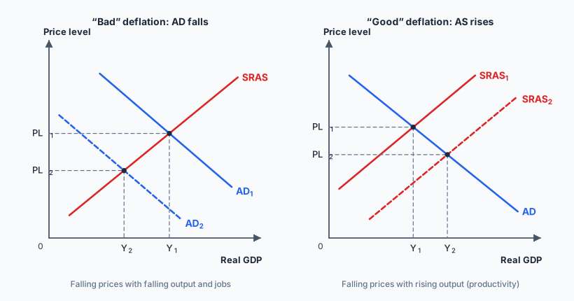
Costs of deflation: uncertainty; redistribution (the real value of debt rises, hurting borrowers); deferred consumption (consumers wait for lower prices, so AD falls further, a deflationary spiral); association with high cyclical unemployment and bankruptcies; increase in the real value of debt for households, firms and governments; inefficient resource allocation; and policy ineffectiveness, because interest rates cannot fall much below zero. Japan’s long spells of mild deflation from the late 1990s are the standard example.
Unemployment versus inflation: which is worse? Unemployment wastes resources permanently (lost output cannot be recovered) and concentrates the pain on a minority, often the poorest. Moderate inflation spreads a smaller cost across everyone, but high inflation damages the whole economy and hurts the poor, who cannot protect their savings. The answer depends on the rates involved, who is affected and for how long.
4. Sustainable government debt HL
- Budget deficit: in one year, government spending exceeds revenue. Government (national) debt is the accumulated total of past borrowing: each deficit adds to the debt; a surplus can reduce it.
- Measured as a percentage of GDP, because the ability to service debt depends on the size of the economy. Indonesia’s law caps the deficit at 3% of GDP and debt at 60% of GDP (the deficit cap was suspended for 2020–22).
- Costs of high debt: debt servicing costs (interest payments take revenue from schools and hospitals); credit ratings fall if lenders doubt repayment, raising interest costs further (Sri Lanka defaulted in 2022); future taxation and spending: debt must eventually be repaid through higher taxes or lower spending, shifting the burden to future generations; less room for fiscal policy in the next recession.
- Debt is more sustainable when it finances productive investment, when growth exceeds the interest rate, when it is borrowed in the domestic currency, and when institutions are credible.
Conflicts between objectives
- Low unemployment and low inflation HL: the Phillips curve: pushing AD up reduces cyclical unemployment but, near full capacity, raises inflation (demand-pull).
- High growth and low inflation: rapid AD-driven growth beyond potential creates an inflationary gap.
- High growth and environmental sustainability: more output often means more emissions and resource use, unless growth is “green”.
- High growth and equity: growth may reward capital and skills disproportionately, widening inequality.
- The conflicts are not inevitable: supply-side growth (LRAS shifting right) raises output while reducing inflationary pressure.
The Phillips curve HL
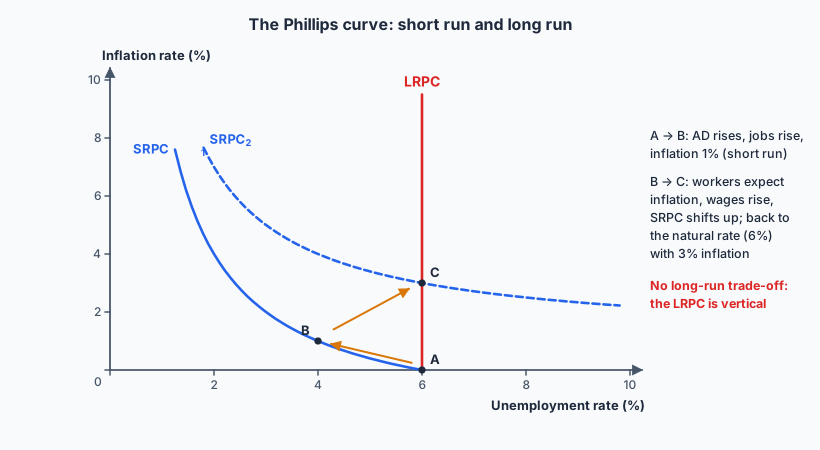
- The short-run Phillips curve (SRPC): A. W. Phillips found (1958) an inverse relationship between unemployment and wage inflation in the UK. It suggested a trade-off: governments could buy lower unemployment with higher inflation by raising AD.
- The 1970s breakdown: stagflation (high inflation and high unemployment) contradicted the simple trade-off.
- The long-run Phillips curve (LRPC): Friedman and Phelps argued that the trade-off is only temporary. When AD rises (A to B), unemployment falls below the natural rate and inflation rises. Workers soon expect higher inflation and demand higher wages, SRAS shifts left, and unemployment returns to the natural rate at the higher inflation rate (C) on a higher SRPC. So the LRPC is vertical at the natural rate of unemployment, which matches the vertical LRAS.
- Implication: demand-side policy cannot permanently reduce unemployment below the natural rate; only supply-side policies can lower the natural rate itself.
✏️Worked example
(b) The CPI rises from 131.5 to 137.8. Calculate the inflation rate.
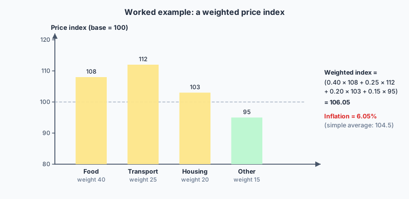
(c) HL A simplified basket has four categories with weights and this year’s price indices (last year = 100): food, weight 40, index 108; transport 25, 112; housing 20, 103; other 15, 95. Calculate the weighted price index and the inflation rate, and compare with a simple average.
(a) 5.1 ÷ 96 × 100 = 5.3%. (Use the labour force, not the working-age population.)
(b) (137.8 − 131.5) ÷ 131.5 × 100 = 6.3 ÷ 131.5 × 100 = 4.8%.
(c)
Inflation = 6.05%. A simple average of the four indices would be (108 + 112 + 103 + 95) ÷ 4 = 104.5, i.e. 4.5%, understating inflation, because the fastest-rising items (food and transport) take the largest share of spending.
📝Practise
Tagged questions are modelled on a real IB question from that session, with our own wording, numbers and context.
1. [10 marks, Paper 1 (a) — modelled on May 2024 SL Paper 1 Q2(a)] Explain, with diagrams, why a consumer boom and a sharp rise in oil prices both raise the price level but have opposite effects on real output.
2. [10 marks, Paper 1 (a) — modelled on May 2023 HL Paper 1 Q2(a)] Explain why an economy producing at its full employment level of output still has some unemployment.
3. [10 marks, Paper 1 (a) — modelled on May 2023 SL Paper 1 Q2(a)] Explain why a prolonged fall in the price level can lead to rising unemployment and more bankruptcies.
4. [10 marks, Paper 1 (a) — modelled on November 2023 HL Paper 1 Q2(a)] Explain why the inflation rate shown by the CPI may differ from the rise in living costs experienced by a retired couple in a rural village.
5. [15 marks, Paper 1 (b) — modelled on November 2022 HL Paper 1 Q2(b)] Using real-world examples, examine whether a government can permanently lower unemployment by accepting a higher rate of inflation.
SRPC: explain the trade-off with AD/AS (rising AD reduces cyclical unemployment and raises demand-pull inflation) and the SRPC diagram. Evidence: many economies saw inflation rise as labour markets tightened in 2021–22.
LRPC (HL): expectations adjust, so unemployment returns to the natural rate: vertical LRPC; no long-run trade-off. 1970s stagflation; cost-push shocks raise both inflation and unemployment together (2022 energy shock).
Evaluation: the trade-off depends on the time frame, on the cause of inflation (demand-pull versus cost-push), on how expectations are formed (credible central banks keep them anchored), and on whether supply-side policies shift the natural rate. Conclude with a justified judgment.
6. [15 marks, Paper 1 (b) — modelled on May 2023 SL Paper 1 Q2(b)] Using real-world examples, discuss whether a government facing both 8% inflation and 8% unemployment should deal with inflation first.
Inflation worse: affects everyone; uncertainty and lower investment; erodes savings and fixed incomes; export competitiveness; hyperinflation can destroy an economy (Zimbabwe, Venezuela); once expectations rise it is costly to reduce.
Unemployment worse: permanent loss of output; concentrated personal, social and economic costs; skills lost (hysteresis); poverty and crime; youth unemployment scars careers.
Judgment: depends on the rates (2% inflation versus 80%; 4% unemployment versus 25%), on duration, on who is affected, and on the country’s safety nets. Many economists would say moderate unemployment is the more serious human cost, but uncontrolled inflation the greater systemic risk.
🔗Go deeper — other people’s work
These are external resources, not mine. If one stops working, tell me and everything above it on this page still stands.
- Badan Pusat Statistik (BPS) — monthly CPI releases with the weights of each expenditure group, and the labour force survey (Sakernas).
- Bank Indonesia — inflation targets and the inflation report.
- IMF World Economic Outlook database — growth, inflation, unemployment and government debt for every country.